
The Direct Sampling (DS) multiple-point simulation method
Recent advances in the domain of geostatistical simulations include multiple-points simulation methods (MPS), which infer spatial structures from conceptual example images, namely training images. Their main advantage is to allow using high-order spatial statistics (as opposed to traditional two-point statistics), that can represent a wide range of spatially structured, low entropy phenomena.
The direct sampling (DS) is a novel MPS algorithm that is drastically simplified compared to previous approaches and has more possibilities. It produces conditional realizations honoring the high-order statistics of uni- or multivariate training images. In addition to having virtually no RAM requirement, the method is straightforward to parallelize. Hence it is computationally efficient and can produce very large and complex realizations.
With the traditional MPS approaches, the training image is usually scanned and all pixels configurations of a certain size (the template size) are stored in a catalogue of data events having a tree or a list structure. This structure is then used to compute the conditional probabilities at each simulated node. Since the memory load increases dramatically with the size of the template and the number of facies, the use of MPS is generally restricted to relatively small problems with limited structural complexity. Moreover, the template is often not large enough to capture large-scale structures, and multi-grids have been introduced to palliate this problem by simulating the large-scale structures first, and later the small-scale features. Limited memory usage restricts the approach to the simulation of univariate fields.
The DS algorithm takes a different approach. Instead of counting and storing the configurations found in the training image, it directly samples the training image for a given data event. The method is based on a sampling method introduced by Shannon (1948), strictly equivalent to the original MPS algorithm of Guardiano and Srivastava (1993), but that does not explicitly need to compute conditional probabilities and therefore does not need to store them. Starting from an initial randomly located point, the training image is scanned. For each of the successive samples, the distance between the data event observed in the simulation and the one sampled from the training image is calculated. If the distance is lower than a given threshold, the sampling process is stopped and the value at the central node of the data event in the training image is directly used for the simulation. Since nothing is stored, neighborhoods can have virtually any size and are not restricted to a template, making the use of multiple-grids unnecessary. In fact, multiple-grids are replaced by a continuous variation in the size of data events during the simulation process. This reduces artifacts and leads to a simpler implementation.
Similarly to other methods, DS can reproduce the structures of complex training images and deal with a wide range of non-stationary problems. Additionally, it can simulate both discrete and continuous variables by choosing specific distances between data events, and can deal with specific cases of non-stationarity. But the richest feature of DS is that multivariate data configurations can be considered, allowing to generate realizations presenting a given multivariate multiple-point dependence. The ability to treat multiple variables simultaneously in a multiple-point framework allows co-simulation without formulating the dependency between the simulated attributes. Instead, the multiple-point dependence is reproduced as it is in the multivariate training image.
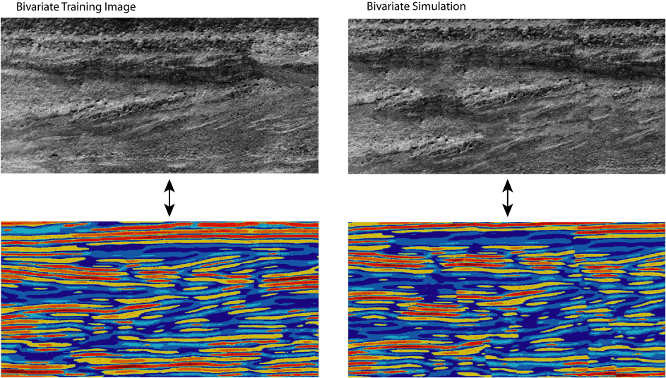
Figure 1: Multivariate training image and one corresponding multivariate simulation
An example is shown in figure 1. The left images represent a bivariate training image consisting of the photograph of an outcrop and a georadar image taken at the same location. The dependence between both variables is shown by the double-headed arrow. One bivariate realization is displayed on the right. Note that the top right image is not an actual photograph, but a simulation of what the photograph could be. Similarly, the bottom right image is a simulation of a georadar image. The dependence between variables is preserved (double-headed arrow), since the simulated photograph of the outcrop presents interfaces at locations that are coherent with the interfaces in the simulated georadar image.
Ressources
- A Matlab example
- Powerpoint presentation: DS_demo.ppt
- A commercial implementation of the direct sampling is available here.
- Guide on the parameterization of DS here.
- Acceleration of DS by simulating patches instead of pixels.
- Here is a set of small Matlab geostatistical tools that you can download and use freely. A basic documentation is also included. Thanks for sending feedback!
References
Mariethoz Grégoire, 2009, Geological stochastic imaging for aquifer characterization. University of Neuchâtel, Centre for Hydrogeology. PhD thesis in Hydrogeology, 225 p. phd_mariethoz2009.pdf