Abstract : During the past 20 years, the fast development of several remote sensors (e.g. Optical imaging, LIDAR, RADAR, etc.) assembled on satellite, aerial or terrestrial platforms is changing our perception and analysis of the Earth’s surface processes. Particularly, LIDAR technology is capable of acquiring faster, denser and more precise information about land terrain surface, allowing the 3D geometrical modelling of mountains, valleys and cliffs at different scales and with an unprecedented level of detail. Consequently, LIDAR applications on landslide mapping, characterization, monitoring and modelling are shedding a light into how landslides behave and evolve along space and time. Some examples include: (1) the precise landslide mapping through the identification of geomorphological features, (2) the accurate extraction of discontinuities characteristics that play a key role in slope stability, (3) the monitoring of landslides in order to analyse 3D displacements, (4) the magnitude/frequency quantification of fallen volumes along time in order to study erosion rates, (4) the improvement of rockfall hazard assessment, (5) the modelling of mass movements run-out, etc.
Keywords : LIDAR, Laser scanner, landslide, mapping, monitoring, structural analysis.
Jaboyedoff, M., Abellán, A., Carrea, D., Derron, M.H., Matasci, B. and Michoud, C., 2018. Mapping and monitoring of landslides using LiDAR. In Natural Hazards (pp. 397-420). CRC Press. DOI : 10.1201/9781315166841-17
Introduction
During the last decades, the research on surface processes has taken its lead from two main developments: (1) faster and more portable remote sensing devices and (2) more powerful computer processors and graphic capabilities. One of these remote sensing techniques the light detection and ranging (LIDAR, all acronyms are found in Table 1), also known as laser scanner – has provided detailed and accurate topographic surveys since the beginning of the twenty-first century (Carter et al., 2001). LIDAR allows us to acquire more than 10.000 points per second from fixed or moving positions, leading to huge sets of data in a three-dimensional (3D) Cartesian coordinate system (i.e. X, Y, and Z coordinates), normally referred to as “point clouds”. This detailed and accurate representation of the terrain surface has been extensively used to characterize, monitor and model landslides (Rowlands et al. 2003; Mc Kean and Roering, 2004; SafeLand Deliverable 4.1. 2010; Jaboyedoff et al., 2012; Abellán et al., 2014).
The two main categories of LIDAR for mapping and monitoring landslides are static and mobile devices. Static devices are commonly named ground-based LIDAR or terrestrial laser scanners (TLSs). Regarding mobile devices, the different instruments are normally classified depending on the platform configuration: either boats (Alho et al., 2009, Michoud et al. 2015), cars (Lato et al., 2009) or flying devices (Shan and Toth, 2008). The latter, also known as airborne laser scanners (ALSs), include LIDAR assembled on airplanes, but the device can also be mounted over unmanned aerial vehicles (UAVs), and helicopters, and can be adjusted to the shooting direction (Vallet and Skaloud, 2004, Li et al. 2011). Examples of point cloud density that can be derived from TLS systems normally range from 100 to 500 points/m2, whereas ALS systems range from 0.5 to 50 points/m2.
Point clouds can be converted to surfaces through different surface reconstruction processes, usually involving Delaunay triangulation. For instance, the point cloud produced by ALS is normally transformed into digital elevation models (DEMs) or high-resolution DEM (HRDEMs), which provide very detailed geomorphological information (Chigira et al., 2004; Ardizzone et al., 2007).
The main achievements on the application of the LIDAR technique to landslide investigations include: (1) the improvement of landslide mapping and inventories using HRDEM (Abdulwahid and Pradhan, 2017); (2) a complete characterization of the 3D slope deformation and signs of precursory activity, allowing the forecasting of landslides failures (Rosser et al., 2007; Collins and Sitar, 2008; Abellan et al., 2010; Pedrazzini et al., 2011); (3) an accurate and detailed monitoring of rock failures (Rosser et al. 2005; Teza et al. 2007; Collins and Sitar 2008; Oppikofer et al. 2008; Prokop and Panholzer 2009; Abellan et al. 2010; Kromer et al. 2017; Caudal et al. 2017); (4) the improvement in rock slope characterization in inaccessible areas thanks to the automatic extraction of discontinuity orientation (Bornaz et al., 2002; Kemeny and Turner, 2008; Gigli and Casagli, 2011, Riquelme et al. 2014); and (5) the identification of geomorphic signatures of debris flows based on HRDEM and accurate erosion and deposit quantification (Cavalli and Marchi, 2008; Bremer and Sass, 2012).
Lidar and laser scanning techniques
1. History
The history of LIDAR technology is directly linked to the Light Amplification by Stimulated Emission of Radiation (LASER) evolution. In 1957, the physicists Charles Townes and Arthur Shawlow at Bell Labs investigated the development of optical Microwave Amplification by Stimulated Emission of Radiation (MASER), which later on became LASER in 1959 (Brooker, 2009). In May 1960, the first instrument which successfully produced a series of pulsed lasers was designed (Hecht, 1994). Less than one year later, the first LIDAR was manufactured for military purposes (Brooker, 2009). Then in the seventies, laser technologies became generalized for civilian applications such as surveying. Some examples include the use of electronic distance meter (EDM) in quarries and tunnel environments (Dallaire, 1974; Petrie, 1990; Petrie and Toth, 2009a).
At the same time, first ALS systems were able to measure the range of the emitted pulse with a precision of 1 m (Miller, 1965; Krabill et al., 1984), for altimetry and bathymetry purposes (Sheperd, 1965; Hoge et al., 1980,). Nevertheless, this technology was limited by the poor accuracy on the position and orientation of the airplane given by the Inertial Navigation Systems (INS). Afterwards, laser devices became more accurate, less heavy, less expensive and eye-safe. Moreover in the early nineties, the improvements on the navigation satellite constellations GPS-NAVSTAR (USA) and GLONASS (USSR) allowed for the overcoming of the limitations of former INS, considerably improving the ALS accuracy (Petrie and Toth, 2009b; Beraldin et al., 2010). In the late nineties, theoretical and practical aspects of ALS techniques were well known and several important works were published (Baltsavias, 1999a; Wehr and Lohr, 1999). Early applications of ALSs consisted in the production of DEM (Baltsavias, 1999b; Carter et al., 2001), the mapping of topographical changes of Greenland’s ice sheet (Krabill, et al., 1995), and the creation of a 3D model of an urban environment (Haala and Brenner, 1999). The mapping and modelling of landslides from HRDEM at regional scale started at the beginning of the twenty-first century century (Haugerud et al., 2003; Schulz, 2004, 2007; Van Den Eeckhaut et al., 2007; Haneberg et al., 2009).
During the last decade, the Geoscience Laser Altimeter System (GLAS) sensor illuminated the Earth with three lasers. One of these sensors was especially designed to monitor different environmental variables, such as polar ice sheet mass balances, vegetation canopy and land elevation with a vertical accuracy of 3 cm (Zwally et al., 2002; Abshire et al., 2005; Schutz et al., 2005). One of the most relevant topographic products derived from the ICESat mission was the 500 m pixel resolution DEM of Antarctica (DiMarzio, 2007; Shan and Toth, 2008). Meanwhile, a space-borne EDM device named Mars Orbiter Laser Altimeter (MOLA) was developed to observe Mars from 1999 to 2001 in order to survey its topography and atmosphere (Smith et al., 2001). This sensor measured the surface of Mars during 15 months, obtaining a DEM of Mars with a resolution of a few square kilometres and a vertical accuracy of 1 m (Smith et al., 2001).
At the same time, pioneering triangulation-based TLS systems were designed and used for archeological purposes (Beraldin et al., 2000). Later on, ground-based LIDAR sensors have been used for surveying and monitoring deformations of urban structures (Gordon et al., 2001; Lichti, et al., 2002). Geological applications of TLSs have been experiencing fast developments since 2002, including: (1) extraction of orientations and roughness of rock slope discontinuities (Slob et al., 2002; Kemeny and Post, 2003; Fardin et al., 2004; Feng and Röschoff, 2004; Jaboyedoff et al., 2007; Sturzenegger and Stead, 2009; Garcia-Selles et al., 2011; Riquelme et al., 2014; ); (2) monitoring of volcanic activity (Hunter et al., 2003); (3) litho-stratigraphic modelling (Bellian et al., 2005; Buckley et al., 2008; Kurz, et al., 2008; Humair et al. 2015); (4) detection of rockfalls (Lim et al., 2005; Rosser et al., 2005; Collins and Sitar, 2008; Abellan et al., 2010); and (5) landslide monitoring (Teza et al., 2007; Collins and Sitar, 2008; Monserrat and Crosetto, 2008; Fey et al. 2015).
2. Instrument principle
2.1 LiDAR functioning
A LIDAR device consists of a combination of a laser rangefinder and a scanning mechanism which allows for the precise measurement of a distance to a target, and the orientation of the laser beam. The scanner device works through the internal rotation of one or two mirrors and/or the rotation of the whole device. Additional components normally include an electronic unit, an imaging device (e.g. digital camera) and specific software to control the whole system.
There are three main types of LIDAR, corresponding to three different ways of measuring the range; for instance, the distance along the line of sight (LOS) between the sensor and the terrain (see Fig. 1): (1) pulse LIDAR measures the time of flight (TOF) of a laser pulse, (2) phase LIDAR uses phase shift between emitted and received signal and (3) triangulation LIDAR uses a camera to locate the laser spot on the scanned surface (Vosselman and Maas, 2010).
Pulse LIDAR is based on the measurement of the time delay (TOF) of a laser pulse travelling from the source (e.g. TLS) to a reflective target (e.g. ground surface) and back to the source, as follows (Petrie and Toth, 2009a):
d = 1/2 c * Δt
Where d is the range, c is the speed of light in the air (3×10⁸ m/s) and Dt is the TOF. This technique allows for centimetre accuracy measurements at several kilometres’ distance. Phase LIDAR allows for a more precise acquisition (some millimetres), but it only works for short ranges (less than 100m). Phase LIDAR uses a continuous amplitude or/and frequency modulated beam instead of pulses. The range is deduced from the phase shifts between emitted and backscattered signal for a couple of frequencies (Petrie and Toth, 2009a). Triangulation LIDAR estimates the range from two angles: the illumination angle of the laser beam and the observation angle of the camera (Beraldin et al., 2010). With a high accuracy (around 0.1 mm), triangulation LIDAR has very short ranges (less than 5 m). Pulse (or TOF) LIDAR is the main device used for landslide monitoring and mapping, since it is the only one that makes possible acquisitions for ranges longer than 100 m (up to a couple of kilometres for the most advanced sensors). There are few applications of phase and triangulation LIDAR for landslides, such as very detailed characterization of sliding surfaces or analogue modelling in the lab (Carrea et al., 2012).
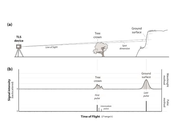
Figure 1: (a) Sketch of LIDAR functioning principle showing TLS device, LOS and spot dimension; (b) Signal intensity vs. TOF for two different methods of measurement: full wavelength method vs. pulse method.
The footprint size depends on the range and the beam divergence angle. The shape of the footprint on the surface depends on the local incidence angle, which is the angle between the LOS and the normal to the surface (Fig. 2). The range is measured at the peak of intensity of the backscattered pulse. If the surface is normal to the laser beam, it corresponds to the centre of the footprint (point P in Fig. 2). If the incidence angle is high (more than 70°) or the local relief is rough, the recorded point of location (point P’ in Fig. 2) can lie anywhere within the spot (Schaer et al., 2007; Lichti and Skaloud, 2010).
2.2 Multiple echoes
Even if strongly collimated, laser beams of LIDARs are affected by divergence; that is, the beam width increases with the range. Typical diameters of beam footprints are 30-50 cm for ALS at 1 km range, and 10 cm for TLS at 500 m range (Lichti and Skaloud, 2010). As a result, the consequences are that several backscattered pulses can correspond to a single emitted pulse (multiple echoes). For instance, when a pulse hits a tree, part of the pulse can be reflected by the top of the canopy, another part by branches and the last one by the ground (see Fig. 2). This characteristic of the beam to “penetrate” the vegetation is a key advantage of LIDAR compared to photogrammetry, in order to get ground elevation models of vegetated areas. However, a dense forest may prevent the beam from reaching the ground surface. Full wave LIDAR devices, usually ALS, provide a continuous record of the backscattered signal (full waveform). Most TLSs record only one or several discrete pulses. In landslide studies, the last pulse, (i.e. the pulse backscattered by the ground surface) is generally used. But it may be convenient to have other return pulses for vegetation removal purposes (Petrie and Toth, 2009a).
2.3 Other parameters: intensity and color
In addition to 3D surface point locations, LIDAR devices measure the signal intensity of the backscattered laser signal. Intensity mainly depends on the type of material, orientation of the slope, range and laser wavelength. Additional external cameras can be coupled with LIDAR during acquisition, allowing the assignment of a color attribute (i.e. RGB) to each point of the LIDAR point cloud. During ALS acquisitions, natural colors and/or infrared images are usually taken simultaneously. A single-lens reflex (SLR) digital camera is frequently used to provide natural colours to TLS point clouds, but more advanced imaging devices, such as hyperspectral cameras, can be used too (Kurz et al., 2011). Some of the main uses of intensity values or colour attributes for landslide studies include bedrock mapping, vegetation removal and interactive visualization of point clouds (Alba et al., 2011).
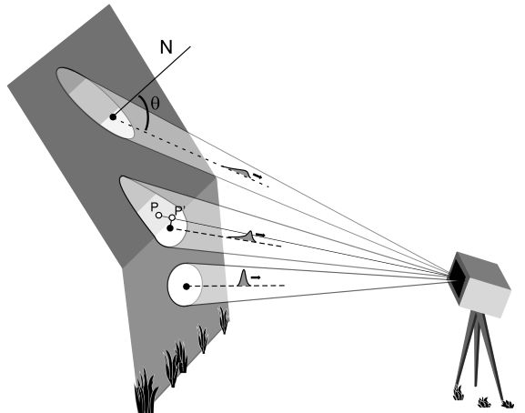
Figure 2. LIDAR footprint deformation (θ , incidence angle; N: normal to the surface). The point position is attributed to the centre of the beam (point P), but the range is measured at the maximum intensity of the backscattered pulse. Then, the actually measured point P’ is located slightly before the rock face on the LOS.
2.4 ALS vs TLS
ALSs are widely used, by either national topography agencies or private companies, to cover large areas for topographical surveying or forest management (Shan and Toth, 2008). The plane usually flies 1000 m above the ground, and the ALS records 1-2 points by ground square-metre (recent developments increase these values by one order of magnitude), with a position accuracy of 5-30 cm (Petrie and Toth, 2009b). Mobile techniques require a precise recording of the location and altitude of the scanning device during the acquisition, which is actually carried out by coupling the LIDAR with a Global Navigation Satellite System (GNSS) (usually a differential global positioning system [GPS]) and with an inertial measurement unit (IMU). Then the location of each point of a scan is recalculated as a function of the LIDAR position and orientation during a post-processing stage. Due to its heavy logistics, ALS is operated by professional surveying companies. Other smaller mobile platforms are also occasionally used for the laser scanning of landslides. For instance, LIDAR sensors can be assembled to helicopters, taking profit of its relatively low flying speed and flying heights close to terrain surface, which allows acquiring 3D information on cliffs from a an oblique view. This was used to scan a 2 km2 area around the Åknes rock slide (Norway), providing 20 measurement points per square meter with a position precision of 5 cm (Blikra et al., 2006; Jaboyedoff et al., 2011). Also, offshore laser scanning from a boat is used for coastal cliff and river bank stability analysis, with a typical average point spacing of 10-20 cm (Alho et al., 2009). Finally, a fast growing technique is the setup of laser scanners on cars or trains in order to acquire high resolution ground models along transport corridors. This technique has been used to assess rock wall stability along roads and railways in Ontario (Canada) with an average point density of 100 points/m2 (Lato et al., 2009).
A TLS is a fixed position scanning technique that only requires the device setup on a tripod opposite the surface to scan within the maximum range limit. Because of this relatively easy implementation, TLS is usually operated directly by geoscientists in charge of the landslide investigation. With a high point density (up to 10,000 points/m2) and accuracy (about 1 cm), it is mostly limited by the availability of a good point of view, the maximum range of acquisition and the relatively small areas that can be covered in single acquisition due to a limited field of view (FOV) angle (for instance, 40° in TLS Ilris3D). Usually, in order to cover the whole area of interest, several scans have to be acquired from different points of view.
2.5 Spacing, accuracy, resolution and data types
The major differences between the two most commonly used techniques (i.e TLSs and ALSs) are: (1) average point spacing: metre scale for ALSs and centimetre scale for TLSs; (2) position and range accuracy: some tens of centimetres for ALS and about 1 cm for TLS; (3) point cloud geometry: as ALSs are usually shooting subvertically, they arevery efficient in order to produce horizontally projected surface, such as gridded DEMs. But it provides a poor representation of steep areas like rock cliffs. In addition to this, as opposed to TLS devices, ALSs are not able to have several ground surface elevation values of ground elevation (Z) for each horizontal position (X, Y), and thus they are unable to represent overhanging walls. Properly speaking, ALS products are 2.5-dimensional (2.5D) elevation surfaces and not full 3D representations of the terrain surface. As a result, most of ALS processing software is inefficient to work properly with point clouds from TLS acquisitions.
Measurement accuracy on single points depends on range, surface reflectivity and incident angle (Ingensand, 2006; Lichti, 2007; Abellán et al., 2009; Lichti and Skaloud, 2010). Inaccuracy of surface location and geometry is due not only to single measurement errors, but also to alignment and merging processes. This is particularly critical when several acquisitions are merged into one dataset. The quality of the final dataset must be carefully checked, because even very small inaccuracies can produce large uncertainties in change detection, as discussed by Schürch et al. (2011).
Point cloud resolution determines the level of detail that can be observed from a scanned point cloud (Pesci et al., 2011), where the laser beam width plays an important role (Lichti and Jamtsho, 2006). However, TLS resolution and point spacing are normally mixed up (Lichti and Jamtsho, 2006). It is recommended to place the optimal point spacing as 86% of the laser beam width at a given distance.
2.6 Data acquisition issues: occlusion and biases
Occlusion: Due to relief roughness and natural variability, the acquisition of rock slope geometry from a single station is normally affected by the existence of shadow areas (also called occluded areas). In order to minimize occlusion issues, (Kemeny and Turner, 2008) different series of best practices and protocols are proposed for survey planning. For instance, occlusion can be minimized using data acquisition from multiple locations (Lato, et al., 2010; Stock et al., 2011).
Biases: Discontinuity characterization may be affected by biases depending on the intersection angle between discontinuity sets and the sensor’s LOS (Sturzenegger and Stead, 2009; Lato, et al., 2010): the density of those families with a normal vector parallel to the LIDAR’s LOS may be over-represented compared to the density of families with a normal vector perpendicular to the LOS of the instrument. Indeed, this is a similar effect observed by Terzaghi, (1962), in which the density of families with directions parallel to the slope orientation may be over represented compared with the families perpendicular to the slope.
3. Data treatment
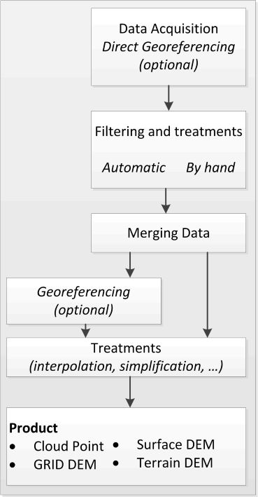
A series of pre-processing steps are necessary in order to transform the RAW LIDAR data (unfiltered point cloud both in ALSs and TLSs) into real terrain points, as follows (see Fig. 3):
3.1 Full-waveform and automatic filtering
The first truly operational full-waveform (FW) LIDAR systems for airborne applications appeared in 1999 (Mallet and Bretar, 2009). This new generation of instruments is able to capture not only the discrete signal return but also the entire waveform. The first experimental full-waveform LIDAR system was originally developed for forestry canopy and building segmentation. At present, full-waveform data are mainly used for ALS applications in order to discriminate the surface terrain from forestry, which is of great interest for vegetation removal and DEM generation. Current research on full-waveform LIDAR data includes signal decomposition for object classification: terrain, vegetation, wires, buildings, and so forth.
The integration of LIDAR-derived 3D data with complementary information registered by other remote sensing methods is also in development. For instance, the coupling of LIDAR and InSAR data was successfully explored for displacement monitoring (Farr et al. 2008; Lingua et al. 2008; Roering et al. 2009). Other spectral attributes provided by multispectral imaging can also help improve interpretation and segmentation of 3D LIDAR data (Kurz et al. 2011).
3.2 Non ground points filtering (including vegetation removal)
Non-ground-point (e.g., vegetation, cables, birds and dust) filtering is a time-consuming task that is commonly performed manually. Although this approach may be straightforward, when non-ground points appear at small portions of the terrain, new semi-automatic methods aiming to classify ground points are being currently developed. These methods of classification, which are normally supervised by the user, are based on the identification of different values of the point cloud that allow us to separate ground from non-ground points. For instance, while some methods use the colour-coded value (RGB) or intensity of the laser return (e.g. Lichti, 2005; Franceschi et al., 2009), other approaches include the study of some geometrical parameters as single point statistics (e.g. Huang et al., 2000), local 3D point cloud statistics (e.g. Lalonde et al., 2006), multi-scale dimensionality criteria (Brodu and Lague, 2012) or using classifiers as support vector machine (Cristianini and Shawe-Taylor, 2000), expectation–maximization (EM) algorithms and/or Gaussian Mixture Models (Xu and Jordan, 1996). Although these methods are highly promising, manual vegetation removal is still currently necessary in most of the cases.
3.3 Point cloud comparison
Point cloud comparison between sequential LIDAR datasets allows the detection of temporal differences in terrain morphology at multiple scales (Lim et al., 2005, Kromer et al., 2015). In order to make a comparison, several steps are required: (1) acquisition of a reference point cloud at initial time (t0); (2) construction of a reference surface at t0; (3) acquisition of successive data point cloud at different time lapses (t1, t2, etc.); (4) co-registration between reference surface and successive data point clouds (Besl and McKay, 1992; Chen and Medioni, 1992); and (5) change detection through the calculation of the differences for each period of comparison.
The single point distances between reference and successive point clouds are normally computed along a user-defined vector in one dimension. This vector can be defined both using a fixed orientation (Rosser et al., 2005; Girardeau-Montaut, 2006) or using different local vectors defined perpendicular to the rock face at each section of the slope, as described in Brodu and Lague (2012). Another method of comparison includes the use of the “shortest distance” between the data point cloud and the reference model. The real 3D deformation of single blocks in terms of rotations and translations can be quantified by using the roto-translational (RT) matrix technique (Collins and Sitar, 2008; Monserrat and Crosetto, 2008). More recently, a series of innovative approaches for surface change detection utilize semi-automatic techniques for 4D investigation of slope failures (Kromer et al. 2015; Williams et al. under review).
Regarding sign criteria, a positive value is normally interpreted as an increase of material (e.g. deposition) or a displacement toward the external part of the slope (pre-failure deformation). Similarly, negative values are normally interpreted as a loss of material on a given period (e.g. soil erosion and rockfalls).
Landslide applications
1. Landslides
Since the beginning of the 2000s, the ALS system has been widely used to produce HRDEMs at regional scale (Petrie and Toth, 2009b). This technique quickly became an essential document of a regional landslide inventory map (Mc Kean and Roering, 2004; Jaboyedoff et al., 2012; Petschko et al. 2016). By creating a hill-shaded surface, it is possible to highlight structures that cannot be seen from aerial photos or in field observations (e.g. Schulz, 2004; Van Den Eeckhaut et al., 2007; Haneberg et al., 2009; Burns et al., 2010) either due to landslide scale (from metric to kilometric), or location (in inaccessible or densely vegetated areas) (Fig. 4). Different approaches are usually employed for landslide mapping and identification, with various degrees of automation: (1) manual or expert-based approach, which focuses on the identification of landslides based on geomorphological evidences of crowns, main scarps, flanks, foot or toe and vegetation cover (Zaruba and Mencl, 1982; Cruden and Varnes, 1996; Soeters and Van Westen, 1996; Agliardi et al., 2001; Braathen et al., 2004); (2) automatic geomorphological features recognition, which extracts different information derived from HRDEMs, such as slope angle, curvature or roughness (Glenn et al., 2006).
When several generations of ALS scans are available, then change detection between HRDEMs can be used to characterize topographic changes. This technique has been employed to detect slope failures, soil erosion, slope displacements and terrain deformation (Burns et al., 2010; DeLong et al., 2012; Fey et al. 2015). Some examples of ALSs for coastal cliff monitoring and erosion analysis are discussed in Young and Ashford (2008) and Reineman et al. (2009). Furthermore, high resolution topography from airborne LIDAR can also be compared with less accurate historical aerial photographs, in order to analyse the kinematics of the landslide over a long-term period.
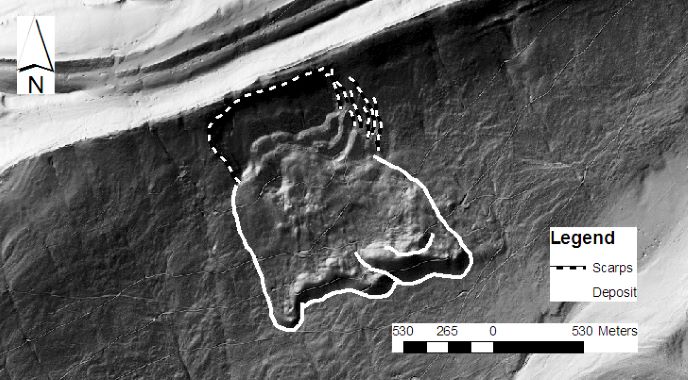
Figure 4. Mapping of a large-scale landslide detected using a LIDAR-based HRDEM. Bern Canton, northwest Switzerland (Data from Géodonnées © Swisstopo, DV084371)
2. Rock slopes
2.1 Structural analysis
The aim of the structural study is the detection and characterization of the main joint sets responsible for the fracturing of the rock mass. The analysis of the network of discontinuities is an essential step to study a rockfall scar or to assess the potential unstable areas of a rock slope. The measurements of the orientation (Fig. 5), undulation, persistence, spacing, opening, roughness and water presence of the main joint sets are usually taken in the field with classical methods, such as photography, direct observations and compass measurements (ISRM, 1978). TLS allows to perform most of these tasks faster, with a high accuracy, and even in inaccessible vertical areas (Kemeny and Post 2003; Jaboyedoff et al. 2009; Lato et al. 2010; Gigli and Casagli 2011; Longoni et al. 2012). Georeferenced 3D TLS point clouds allow us to extract the orientation of structures and to perform distance or volume measurements (Oppikofer et al., 2009; Olsen et al. 2015). Similar results can be obtained from HRDEM generated from aerial LIDAR, but with significant limitations imposed by the vertical shooting direction and by the size of the cells. The representation of structural features like planes or lines, which is classically done with stereoplots (ISRM, 1978), can also be automatically extracted using modern algorithms. Early studies used a manually selected section of the point cloud and calculated the best-fitting plane (Oppikofer et al., 2009; Sturzenegger and Stead, 2009), which can be laborious and time-consuming. Later on, some authors proposed the construction of 2.5D surfaces such as Triangular Irregular Networks (TIN) for the automatic calculation of the discontinuity orientation (Slob et al., 2002; Kemeny and Turner, 2008). More recently, techniques allow automatically computing local plane orientations directly from the point cloud (Ferrero et al., 2009; Garcia-Selles et al., 2011; Gigli and Casagli, 2011; Riquelme et al., 2014). In order to facilitate structural interpretations, the orientation and inclination of each point of a TLS point cloud, or of a DEM cell, can be represented using a unique colour (Jaboyedoff et al., 2007). The resolution of the datasets plays an important role in the analysis of discontinuity orientation: as discussed in Sturzenegger and Stead (2009), low-resolution datasets may lead to (1) a truncation of non-persistent discontinuity sets due to a lack of information and (2) a shifting of discontinuity orientation due to a non-realistic smoothening of the surface geometry.
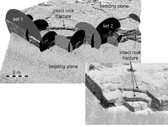
Figure. 5. Discontinuity mapping on a Terrestrial LIDAR point cloud, rendered using greyscale intensity values (From Sturzenegger and Stead, 2009; with permission)
2.2 Monitoring of fragmental rockfalls
Due to the steepness of rock slopes, terrestrial LIDAR is more extensively used than airborne LIDAR for the monitoring of fragmental rockfalls. Moreover, terrestrial LIDAR provides an unprecedented level of detail at a site-specific slope, both resolution and accuracy ranging from several millimetres to a few centimetres. A pioneer approach for monitoring fragmental rockfalls along a section of marine cliffs in northeast England was developed by Lim et al. (2005) and Rosser et al., (2005). Since then, TLSs have become a widely used tool for automatic rockfall detection and volume calculation (Abellan et al., 2010; Stock et al., 2011; Collins and Stock, 2012; Carrea et al. 2014; Tonini and Abellan, 2014; Micheletti et al. 2017; Williams et al. under review). Using the TLS technique, Stock, et al., (2012) detected a series of progressive rockfalls that occurred in exfoliated granitic rocks, analysing how a given fracture event initiated subsequent adjacent failures. A common application of TLSs for rockfall monitoring includes the analysis of Magnitude-Frequency (MF) characterization of fragmental rock falls. Indeed, several authors have observed a scale-invariant pattern in a MF dimension under log-log scale (Rosser et al., 2005; ; Dewez et al., 2009; Lim et al., 2010; Santana et al., 2012) (Fig. 6), suggesting that a self-organized criticality (SOC) may rule rockfall phenomena (Hergarten, 2003). Some other applications include the monitoring of several million cubic metres of rockslides (Fig. 7) in order to quantify deformation rates and failure mechanisms (Collins and Sitar, 2008; Avian et al., 2009; Oppikofer et al., 2009; Ravanel et al., 2010), and the failure forecasting based on a given precursory indicator: either minor scale rockfalls or tertiary creep deformation (Rosser et al., 2007; Abellan et al., 2010; Royan et al., 2013; Kromer et al. 2017). More recently, the combination of web-retrieved images and LIDAR data for rock slope monitoring has been explored (Guerin et al. 2017; Voumard et al. 2017).
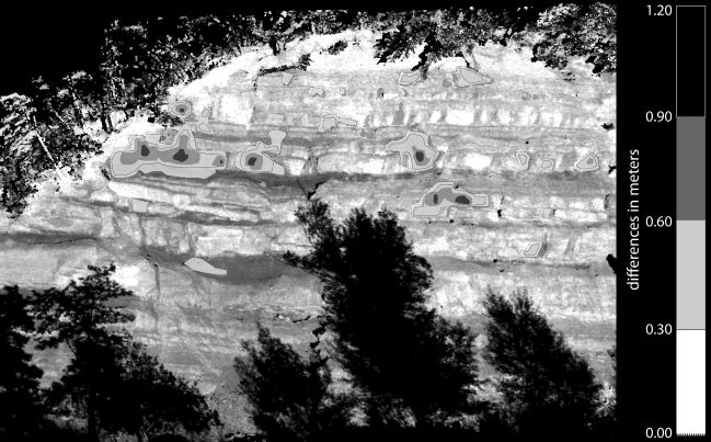
Figure 6. Model comparison showing the changes (i.e., rockfalls) along time on La Cornalle study area (Vaud, Switzerland)(2) .
2.3 Rockfall susceptibility assessment
The simplest way to detect the potential rockfall source areas is by defining a slope angle threshold above which rockfalls are more susceptible to occur (Guzzetti et al., 2003). This method can be optionally coupled with other criteria such as the presence of cliff areas (Jaboyedoff and Labiouse, 2003). The slope threshold can be gathered from a detailed statistical analysis of slope angles, thus allowing to identify the cliff area (Strahler, 1954; Baillifard et al., 2004; McKean and Roering, 2004; Loye et al. 2009). A simple GIS approach developed by Baillifard et al. (2003) allows identifying potential rockfall source areas along roads according to the presence or absence of four parameters: faults, scree slopes, rock cliffs, and steep slopes. A great improvement related to the use of DEMs for the detection of rockfall-prone areas consists in the automatic realization of a kinematic analysis along the whole area (Wagner et al., 1988; Gokceoglu et al., 2000). This analysis allows the detection the topography areas where a discontinuity of a given orientation can lead to an instability. Using a standard classic stability criterion (Norrish and Wyllie, 1996) together with a statistical analysis of the kinematic tests, Gokceoglu et al. (2000) were able to produce probability maps of different failure mechanisms such as planar sliding, toppling and wedge sliding. The kinematic analysis criterion was applied to accurately detect the most unstable areas from TLS data (Fanti et al., 2013). Spacing and persistence of the joint sets, which can be determined both in the field and on LIDAR point clouds (Sturzenegger and Stead, 2009; Lato, et al., 2010; Riquelme et al. 2015), should also be taken into account in the stability calculations, as suggested by Jaboyedoff et al. (2004). The number of potential failures per cliff area can be calculated based on the spacing and on the trace length values, which considerably improves the rockfall susceptibility maps (Brideau et al., 2011; Matasci et al. accepted).
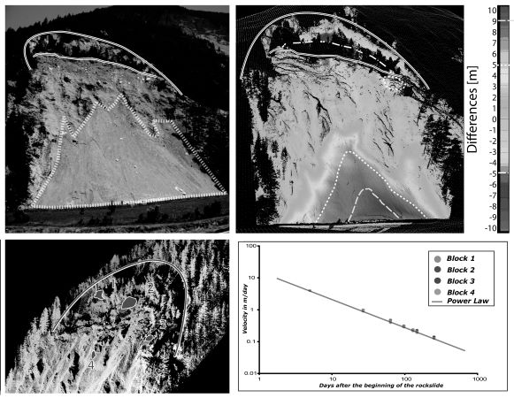
Figure 7. Different techniques for the quantification of a mass movement located on Montatuay mountain (Valais, Switzerland) using a ground-based LIDAR. (a) Picture of the study area; (b) Filtered point cloud of the study area; each point is coloured according to the differences calculated between the 2009 ALS DEM and the TLS point cloud captured in April 2011. (c) Rotated perspective of the LIDAR point cloud, including the manual selection of different blocks for subsequent tracking. (d) Velocity computation for each of the previously selected blocks; the straight line in log-log scale shows a progressive stabilization of the slope.
3. Debris flows
LIDAR is used for various tasks related to debris flows mapping, characterization and modelling. HRDEMs from ALSs are frequently used to identify and characterize initiation and propagation zones of debris flows (Staley et al., 2006; Conway et al., 2010; Lopez Saez et al., 2011; Lancaster et al., 2012) anddeposition fans (Staley et al., 2006), or to estimate the eroded and deposited volumes (Breien et al., 2008; Scheidl et al., 2008; Bull et al., 2010). Remarkably, Schürch et al. (2011) have used TLSs to detect surface changes along a debris flow channel in Switzerland, and Cavalli and Marchi (2008) have combined TLS and ALS to quantify sediment transport for debris flow events in the Austrian Alps, observing several metre changes between the two epochs (Fig. 8). ALS data are also used to estimate the volume of sediments that can be potentially entrained along the channels by a future event (Abancó and Hürlimann, 2014). Apart from geomorphic analysis, a DEM from laser scanning can also be used in debris flow propagation modelling. For instance, Stolz and Huggel (2008) have assessed the impact of HRDEM cell sizes (1, 4 and 25 m.) on modelled propagations, in particular the effect of resolution on debris flow confinement along recent channels.
4. Input for modelling
Mass movement modelling is the process of simulating its stability and/or its propagation across time. This analysis can be carried out using conventional representations of a terrain’s surface, either DEM or HRDEM. Note: current models do not utilize real 3D point clouds but 2.5D projections of the topography.
One of the first applications of LIDAR topographic data for landslide modelling was presented by Dietrich et al. (2001) using the SHALSTAB model. These authors showed that susceptibility mapping of shallow landslides can be considerably improved when using a HRDEM of 1 m cell size obtained from ALS. The results of this simulation demonstrated that the distribution of potentially unstable areas was closer to the inventoried landslides than when using low resolution DEM. In addition, the total surface of affected terrain was smaller. The same trend has also been observed in other available models such as TRIGRS, which includes more sophisticated infiltration models (Savage et al., 2003; Godt et al., 2008).
The optimal accuracy and resolution of the DEM for modelling should be carefully considered. Although HRDEM usually improves the modelling of the phenomena, most of the conventional modelling packages do not necessarily require more than a 5 to 10 m DEM resolution (Liao et al., 2011). Modelling using a higher resolution DEM can even introduce artefacts and non-realistic noises that can mask the main terrain features (Tarolli and Tarboton, 2006). For instance, ALS derived DEM used for mapping debris flow kinematics have a strong dependency on lateral spreading on the DEM resolution (Stolz and Huggel, 2008; Horton et al., 2013). It was found that the fine resolution produced geometric artefacts, degrading the quality of the modelling results. Similarly, the use of HRDEMs for the simulation of rockfall propagation can lead to significant differences when compared with lower resolution DEMs (Agliardi and Crosta, 2003; Janeras et al., 2004). For instance, the lateral dispersion of the trajectories and the kinetic energy vary with DEM resolution that controls the roughness of the terrain surface (Agliardi and Crosta, 2003). According to Agliardi and Crosta (2003), the maximum kinetic energy normally increases with the DEM resolution. However, the opposite result is presented in Jaboyedoff et al. (2006). This discrepancy may be explained by the fact that a higher resolution DEM has little impact on the accuracy of the results when other parameters (geology, vegetation, etc.) are poorly described (Fuchs et al., 2014). The resolutions of the LIDAR DEM are often too fine compared to the other required input data (Brideau et al., 2011).
Erosion and hillslope evolution modelling has been greatly enhanced by using HRDEM (Roering, 2008; Neugirg et al. 2016). However, most of the current packages for landslide modelling are not able to make the best use of high-resolution LIDAR data. The increasing power of computers will certainly lead to an extensive use of HRDEM as input for stability and run-out modelling. One can expect that the exploitation of full 3D data will be attained in the near future.
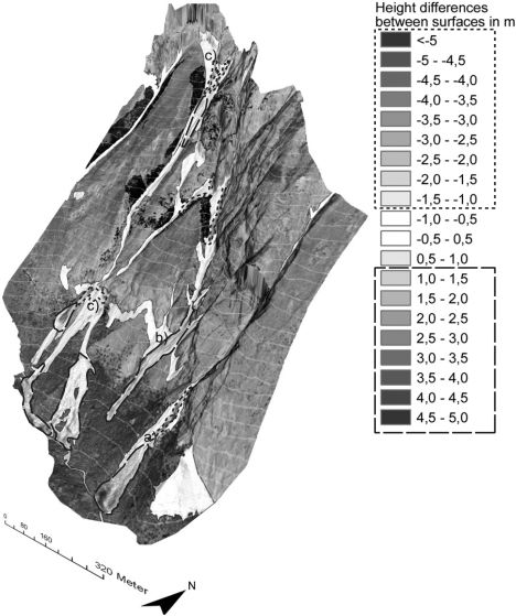
Figure 8. Surface differences between pre-event (ALS) and post-event (TLS) datasets (negative values for erosion). ( From Bremer and Sass, 2012; with permission).
Conclusion
The current knowledge concerning the mapping and monitoring of landslides is now far beyond what was expected by the end of the nineties. This is mainly due to the recent advances in remote sensing techniques (including LIDAR) together with the exponential growth of computational capabilities. For instance, laser scanning has allowed for the development of new techniques to monitor slope changes and slope movements, providing innovative ways for hazard qualification and a better understanding of the surface processes such as rockfall failures.
Dense 3D data has become popular thanks to LIDAR. Nevertheless, one of the present-day key issues is the scarce software to extract all the landslide-relevant information from the unprocessed LIDAR data, especially from full waveform data. At present, different modelling techniques benefit only partially from the full resolution of the LIDAR derived DEMs. This is linked to the fact that the density and the quality of the geometrical information are much higher than other parameters required for hazard assessment, such as geological maps. Despite this, the recent advances achieved on the study of rockfalls, and rock slopes indicate that HRDEMs possess a great potential for the development of new methods and techniques for the analysis of landslide phenomena.
New applications and techniques are now emerging and will be used as a routine in a near future: (1) the development of new algorithms for the analysis of complex slope deformations in space and time (Kromer et al. 2015; Williams et al. under review); (2) the detection of slope movement in real-time and its integration on early warning systems (Olsen et al., 2012; Kromer et al. 2015; Williams et al. under review); (3) the possibility to rapidly acquire accurate 3D data along transport corridors using mobile mappers (Fig. 9); (4) the improvement of TLS technical capabilities, including maximum range, accuracy and point density; (5) the merging of web-retrieved images and terrestrial LIDAR data for slope monitoring (Guerin et al. 2017; Voumard et al. 2017); (6) the acquisition of Earth surface topography by a new generation of satellite LIDAR such as ICESat-2 planned for 2018 and (7) the releasing of LIDAR data to the public domain in open repositories, including ‘Open Topography’ and ‘Point Cloud Library’ is helping raising awareness on the importance of 3D and 4D data treatment.
In conclusion, we can say that LIDAR technology has completely revolutionized the characterization, mapping and monitoring of landslides during the last decades. However, a series of great challenges still remain on the development of innovative tools to rapidly extract geohazard related information from LIDAR data.
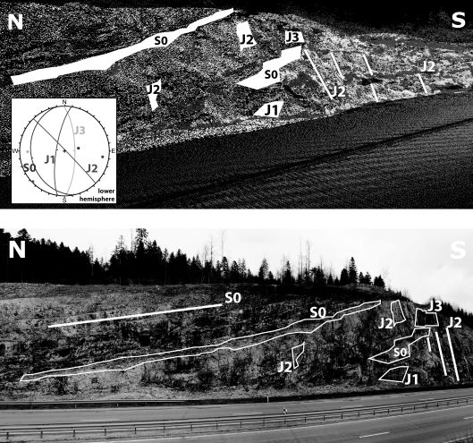
Figure 9. (a) Example of discontinuities mapping along a highway at Pontarlier (East France) using an Optech Lynx Mobile Mapper LIDAR. (b) Picture of the study area.
Acknowledgements
The present work has been partially supported by the Swiss National Foundation project numbers 138015 (Understanding landslide precursory deformation from superficial 3D data), 127132 (Rockfall sources: toward accurate frequency estimation and detection) and 144040 (Characterizing and analysing 3D temporal slope evolution). In addition, the second author was funded by the H2020 Program of the European Commission during manuscript review [Ref: MSCA-IF-2015-705215].
References
Abancó, C. and Hürlimann, M. (2014). Estimate of the debris-flow entrainment using field and topographical data. Natural Hazards, 71(1), 363-383.
Abdulwahid, W. M., and Pradhan, B. (2017). Landslide vulnerability and risk assessment for multi-hazard scenarios using airborne laser scanning data (LIDAR). Landslides, 14(3), 1057–1076
Abellán, A., Jaboyedoff, M., Oppikofer, T. and Vilaplana, J.M. (2009). Detection of millimetric deformation using a terrestrial laser scanner: experiment and application to a rockfall event. Nat. Hazards Earth Syst. Sci., 9, 365–372.
Abellán A., Vilaplana J.M., Calvet J. and Blanchard J. (2010). Detection and spatial prediction of rockfalls by means of terrestrial laser scanning modelling. Geomorphology, 119, 162-171.
Abellán, A., Jaboyedoff, M., Oppikofer, T., Rosser, N.J., Lim, M. and M. Lato (2014). State of Science: Terrestrial Laser Scanner on rock slopes instabilities. Earth surface proc. and landforms, 39, 1, 80-97 . DOI: 10.1002/esp.3493
Abshire, J.B., Sun, X., Riris, H. , Sirota, J.M., McGarry, J.F., Palm, S., Yi, D., Liiva, P. (2005). Geoscience Laser Altimeter System (GLAS) on the ICESat Mission: On-orbit measurement performance. Geophysical Research Letters, Vol. 32.
Agliardi, F., Crosta, G., Zanchi, A. (2001). Structural constraints on deep-seated slope deformation kinematics. Engineering Geology, 59, 83–102.
Agliardi, F. and Crosta, G.B. (2003). High resolution three-dimensional numerical modelling of rockfalls. Int. J. Rock Mecha. Mining Sci., 40, 455–471. DOI:10.1016/S1365-1609(03)00021-2.
Alba, M., Barazzetti, L., Roncoroni, F. and Scaioni, M. (2011). Filtering vegetation from terrestrial point clouds with low-cost near infrared cameras, Italian Journal of Remote Sensing, 43, 55-75.
Alho P., Kukko A., Hyyppä H., Kaartinen H., Hyyppä J. and Jaakkola A. (2009). Application of boat-based laser scanning for river survey, Earth Surf. Process. Landforms, 34, 1831-1838.
Ardizzone, F., Cardinali, M. and Galli, M. (2007). Identification and mapping of recent rainfall-induced landslides using elevation data collected by airborne LIDAR. Nat. Hazards Earth Syst. Sci., 7, 637–650.
Avian, M., Kellerer-Pirklbauer, A., and Bauer, A. (2009). LIDAR for monitoring mass movements in permafrost environments at the cirque Hinteres Langtal, Austria, between 2000 and 2008, Nat. Hazards Earth Syst. Sci., 9, 1087-1094, DOI:10.5194/nhess-9-1087-2009.
Baillifard, F., Jaboyedoff, M., and Sartori, M. (2003). Rockfall hazard mapping along a mountainous road in Switzerland using a GIS-based parameter rating approach, NHESS, 3, 435–442.
Baillifard, F., Jaboyedoff, M., Rouiller, J.-D., Couture, R., Locat, J., Robichaud, G., and Gamel, G. (2004). Towards a GIS-based hazard assessment along the Quebec City Promontory, Quebec, Canada., in: Landslides Evaluation and stabilization, edited by Lacerda, W., Ehrlich, M., Fontoura, A., and Sayão, A. A., pp. 207 – 213, Balkema.
Baltsavias, E.P. (1999a). Airborne laser scanning: basic relations and formulas. ISPRS Journal of Photogrammetry & Remote Sensing, 54, 199-214.
Baltsavias, E.P. (1999b). A comparison between photogrammetry and laser scanning. ISPRS Journal of Photogrammetry & Remote Sensing, 54, 83-94.
Barbarella, M., Fiani, M., and Lugli, A. (2017). Uncertainty in terrestrial laser scanner surveys of landslides.Remote Sensing, 9(2), 113.
Bellian, J.A., Kerans, C., Jennette, D.C. (2005). Digital Outcrop Models: Applications of Terrestrial Scanning LIDAR Technology in Stratigraphic Modeling. Journal of Sedimentary Research, 75 (2), 166-176.
Beraldin, J.-A., Blais, F., Boulanger, P. (2000). Real world modelling through high resolution digital 3D imaging of objects and structures. ISPRS Journal of Photogrammetry & Remote Sensing, 55, 230–250.
Beraldin, J.-A., Blais, F.and Lohr, U. (2010). Laser Scanning Technology. In Airborne and Terrestrial Laser Scanning, Vosselman, G., Maas, H.-G., Eds., Whittles Publishing, Dunbeath, Scotland, 1-42.
Besl, P. and McKay, N. (1992). A method for registration of 3-D shapes. IEEE Transactions on Pattern Analysis and Machine Intelligence, 14, 239-256.
Blikra, L.H., Anda, E., Belsby, S., Jogerud, K. and Klempe, Ø. (2006). Åknes/Tafjord prosjektet: Statusrapport for Arbeidsgruppe 1 (Undersøking og overvaking), Åknes/Tafjord project, Stranda, Norway (in Norwegian).
Bornaz, L., Lingua, A.and Rinaudo, F. (2002). Engineering and environmental applications of laser scanner techniques. Int. Archi. Photogramm. Remote Sens., 34(3B):40–43.
Braathen, A., Blikra, L.H., Berg, S.S., Karlsen, F. (2004). Rock-slope failures in Norway, type, geometry and hazard. Norwegian Journal of Geology, 84, 67–88.
Breien, H., De Blasio, F., Elverhøi, A., Høeg, K. (2008). Erosion and morphology of a debris flow caused by a glacial lake outburst flood, Western Norway, Landslides, 5, 3, 271-280.
Bremer, M. and Sass, O. (2012). Combining airborne and terrestrial laser scanning for quantifying erosion and deposition by a debris flow event. Geomorphology, 138, 1, 49-60.
Brideau M.A., Pedrazzini A., Stead D., Froese C., Jaboyedoff J., van Zeyl D. (2011). Three-dimensional slope stability analysis of South Peak, Crowsnest Pass, Alberta, Canada, Landslides, 8:139–158, DOI 10.1007/s10346-010-0242-8.
Brodu, N. and Lague, D. (2012). 3D terrestrial LIDAR data classification of complex natural scenes using a multi-scale dimensionality criterion: Applications in geomorphology: ISPRS Journal of Photogrammetry and Remote Sensing, 68, 121–134.
Brooker, G. (2009). Introduction to sensing. Introduction to Sensors for Ranging and Imaging, SciTech Publishing Inc.: Raleigh, USA, 1-22.
Buckley, S.J., Howell, J.A., Enge, H.D., Kurz, T.H. (2008). Terrestrial laser scanning in geology: data acquisition, processing and accuracy considerations. Journal of the Geological Society, 165, 625-638.
Bull, J.M., Miller, H., Gravley, D.M., Costello, D., Hikuroa, D.C.H., Dix, J.K. (2010). Assessing debris flows using LIDAR differencing: 18 May 2005 Matata event, New Zealand, Geomorphology, 124, 75–84.
Burns, W. J., Coe, J. A., Kaya, B. S., Ma, L. (2010). Analysis of elevation changes detected from multi-temporal LIDAR surveys in forested landslide terrain in western Oregon. Environmental & Engineering Geoscience, 16 (4), 315-341.
Carrea, D., Abellán, A., Derron, M.H., Gauvin, N., and Jaboyedoff, M. (2012). Using 3D surface datasets to understand landslide evolution: from analogue models to real case study. Proceedings of the 11th International Symposium on Landslides and 2nd North American Symposium on Landslides, June 2-8, Banff, Alberta, Canada.
Carrea, D., Abellán, A., M.-H., Derron, and Jaboyedoff, M. (2014). Automatic rockfalls volume estimation based on Terrestrial Laser Scanning data, International Association Engineering Geology Conference, Sept 15-19, 2014 Torino (Italy).
Carter, W., Shrestha, R., Tuell, G., Bloomquist, D and Sartori, M. (2001). Airborne Laser Swath Mapping Shines New Linght on Earth’s Topography. EOS, 82 (46), 549-564.
Caudal, P., Grenon, M., Turmel, D., and Locat, J. (2017). Analysis of a large rock slope failure on the east wall of the LAB Chrysotile Mine in Canada: LIDAR Monitoring and Displacement Analyses. Rock Mech. Rock Eng., 50(4), 807–824.
Cavalli, M. and Marchi, L. (2008). Characterisation of the surface morphology of an alpine alluvial fan using airborne LIDAR. Nat. Hazards Earth Syst. Sci., 8:323–333.
Chen, Y. and Medioni, G. (1992). Object Modelling by Registration of Multiple Range Images. Image and Vision Computing, 10, 145–155.
Chigira, M., Duan, F., Yagi, H and Furuya, F. (2004). Using an airborne laser scanner for the identification of shallow landslides and susceptibility assessment in an area of ignimbrite overlain by permeable pyroclastics. Landslides, 1, 203-209.
Collins B. and Sitar N. (2008). Processes of coastal bluff erosion in weakly lithified sands, Pacifica, California, USA, Geomorphology, 97, 483–501.
Collins, B.D. and Stock, G.M., (2012). LIDAR-based rock-fall hazard characterization of cliffs. In: Hryciw R.D., Athanasopoulos-Zekkos A., and Yesiller N. (eds.), ASCE Geotechnical Special Publication No. 225, Geotechnical Engineering State of the Art and Practice, , pp. 3021-3030.
Conway, S.J., Decaulne, A., Balme, M.R., Murray, J.B., Towner, M.C. (2010). A new approach to estimating hazard posed by debris flows in the Westfjords of Iceland. Geomorphology, 114, 4, 556-572.
Cristianini, N. and Shawe-Taylor J. (2000). An Introduction to Support Vector Machines: And Other Kernel-Based Learning Methods. Cambridge, England: Cambridge University Press.
Cruden, D.M. and Varnes, D.J. (1996). Landslides investigation and mitigation, transportation research board. In: Turner AK, Schuster RL (eds) Landslide types and process, National Research Council, National Academy Press, Special Report, 247:36–75.
Dallaire, E.E. (1974). Electronic distance measuring revolution well under way, Civil Engineering, 44, 66-71.
DeLong SB, Prentice CS, Hilley GE, Ebert Y. (2012). Multitemporal ALSM change detection, sediment delivery, and process mapping at an active earthflow. Earth Surf. Process. Landforms, 37(3), 262–272. DOI: 10.1002/esp.2234.
Dewez, T., Gebrayel, D., Lhomme, D., Robin, Y. (2009). Quantifying morphological changes of sandy coasts by photogrammetry and cliff coasts by lasergrammetry. La Houille Blanche, (1) 32-37 DOI: 10.1051/ lhb:2009002
Dietrich, W.E., Bellugi, D., Real de Asua, R. (2001). Validation of the shallow landslide model, SHALSTAB, for forest management. In: Wigmosta MS, Burges SJ (eds.) Land use and watersheds: human influence on hydrology and geomorphology in urban and forest areas, Water Science and Application, 2, 195–227.
DiMarzio, J. P. (2007). GLAS/ICESat 500 m Laser Altimetry Digital Elevation Model of Antarctica. Boulder, Colorado USA: National Snow and Ice Data Center.
Fanti R, Gigli G, Lombardi L, Tapete D, Canuti P (2013). Terrestrial laser scanning for rockfall stability analysis in the cultural heritage site of Pitigliano (Italy). Landslides, 10, 409–420. DOI: 10.1007/s10346-012-0329-5.
Fardin, N., Feng, Q., Stephansson, O. (2004). Application of a new in situ 3D laser scanner to study the scale effect on the rock joint surface roughness. International Journal of Rock Mechanics & Mining Sciences, 41, 329–335.
Farr, T.G., Rignot, E., Saatchi, S., Simard, M. and Treuhaft, R. (2008). LIDAR/InSAR Synergism for Earth Science Applications, Synthetic Aperture Radar (EUSAR), 2008 7th European Conference, pp.1-3, 2-5 June 2008.
Feng, Q.H., Röschoff, K. (2004). In-situ mapping and documentation of rock faces using a full-coverage 3-D laser scanning technique. International Journal of Rock Mechanics & Mining Sciences, 41 (3).
Ferrero AM, Forlani G, Roncella R, Voyat HI. (2009). Advanced geostructural survey methods applied to rock mass characterization. Rock Mechanics and Rock Engineering, 42(1), 631–665. DOI: 10.1007/s00603-008-0010-4
Fey, C., Rutzinger, M., Wichmann, V., Prager, C., Bremer, M., and Zangerl, C. (2015). Deriving 3D displacement vectors from multi-temporal airborne laser scanning data for landslide activity analyses. GIScience & Remote Sensing, 52(4), 437–461.
Franceschi, M., Teza, G., Preto, N., Pesci, A., Galgaro, A., Girardi, S. (2009). Discrimination between marls and limestones using intensity data from terrestrial laser scanner. ISPRS J. Photogramm., 64(6), 522-528. DOI:10.1016/j.isprsjprs.2009.03.003.
Fuchs M, Torizin J, Kühn F. (2014). The effect of DEM resolution on the computation of the factor of safety using an infinite slope model. Geomorphology, 224, 16-26, DOI: 10.1016/j.geomorph.2014.07.015.
Garcia-Selles D, Falivene O, Arbues P, Gratacos O, Tavani S, Munoz JA. (2011). Supervised identification and reconstruction of near-planar geological surfaces from terrestrial laser scanning. Computers & Geosciences 37, 1584-1594. DOI: 10.1016/j.cageo.2011.03.007
Gigli, G. and Casagli, N. (2011). Semi-automatic extraction of rock mass structural data from high resolution LIDAR point clouds, Int. J.Rock. Mech. Min., 48, 187–198.
Girardeau-Montaut, D. (2006). Détection de changement sur des données géométriques tridimensionnelles. Doctorat Traitement du Signal et des Images, TSI/TII, ENST, available at: https://pastel.enst.fr/1745
Glenn, N.F., Streutker, D.R., Chadwick, D.J., Thackray, G.D., Dorsch, S. J. (2006). Analysis of LIDAR-derived topographic information for characterizing and differentiating landslide morphology and activity. Geomorphology, 73(1-2), 131-148.
Godt, J.W., Baum, R.L., Savage, W.Z., Salciarini, D., Schulz, W.H., and Harp, E.L. (2008). Transient deterministic shallow landslide modeling: Requirements for susceptibility and hazard assessments in a GIS framework, Engineering Geology, 102, 214-226, DOI: 10.1016/j.enggeo.2008.03.019.
Gokceoglu, C., Sonmez, H., and Ercanoglu, M. (2000). Discontinuity controlled probabilistic slope failure risk maps of the Altindag (settlement) region in Turkey, Eng. Geol., 55, 277–296.
Gordon, S., Litchi, D., Stewart, M. (2001). Application of a High-Resolution, Ground-Based Laser Scanner for Deformation Measurements. In New Techniques in Monitoring Surveys I, Proceedings of the 10th FIG International Symposium on Deformation Measurements, Orange, USA, 23-32.
Guerin, A., Abellán, A., Matasci, B., Jaboyedoff, M., Derron, M. H., and Ravanel, L. (2017). Brief communication: 3-D reconstruction of a collapsed rock pillar from Web-retrieved images and terrestrial LIDAR data—The 2005 event of the west face of the Drus (Mont Blanc massif). Nat. Hazards Earth Syst. Sci., 17(7), 1207.
Guzzetti, F., Reichenbach, P., and Wieczorek, G. F. (2003). Rockfall hazard and risk assessment in the Yosemite Valley, California, USA, NHESS, 3, 491–503.
Haala, N. and Brenner, C. (1999). Extraction of buildings and trees in urban environments. ISPRS Journal of Photogrammetry & Remote Sensing, 54, 130-137.
Haneberg, W.C., Cole, W.F. and Kasali, G. (2009). High-resolution LIDAR-based landslide hazard mapping and modeling, UCSF Parnassus Campus, San Francisco, USA. Bull Eng Geol Environ, 68, 263–276.
Haugerud, R.A., Harding, D.J., Johnson, S.Y., Harless, J.L., Weaver, C.S. and Sherrod, B.L. (2003). High-resolution LIDAR topography of the Puget Lowland, Washington—A Bonanza for earth science. GSA Today, 13:4–10.
Hecht, J. (1994). Understanding Lasers: An Entry Level Guide, 2nd Ed., IEEE Press: New York, USA.
Hergarten, S. (2003). Landslides, sandpiles, and self-organized criticality, Nat. Hazards Earth Syst. Sci., 3, 505-514, DOI:10.5194/nhess-3-505-2003.
Hoge, F.E., Swift, R.N. and Frederick, E.B. (1980). Water depth measurement using an airborne pulsed neon laser system, Applied Optics, 19, 871-883.
Horton, P., Jaboyedoff, M., Rudaz, B., and Zimmermann, M. (2013). Flow-R, a model for susceptibility mapping of debris flows and other gravitational hazards at a regional scale, Nat. Hazards Earth Syst. Sci., 13, 869–885, DOI:10.5194/nhess-13-869-2013.
Huang, J., Lee, A., Mumford, D. (2000). Statistics of Range Images. Paper presented at the IEEE International Conference on Computer Vision and Pattern Recognition 2000 (CVPR’00), Los Alamitos, CA, USA.
Humair, F., Carrea, D., Matasci, B., Jaboyedoff, M., and Epard, J. L. (2015). Stratigraphic layers detection and characterization using Terrestrial Laser Scanning point clouds: Example of a box-fold. Eur. J. of Remote Sens., 48, 541–568.
Hunter, G., Pinkerton, H., Airey, R., Calvari, S. (2003). The application of a long-range laser scanner for monitoring volcanic activity on Mount Etna. Journal of Volcanology and Geothermal Research, 123, 203-210.
Ingensand, H. (2006). Metrological aspects in terrestrial laser-scanning technology. In Proceedings of the 3rd IAG/12th FIG Symposium 2006, Baden, Austria.
ISRM ( International Society for Rock Mechanics) (1978). Suggested methods for the quantitative description of discontinuities in rock masses, International Journal of Rock Mechanics and Mining Sciences & Geomechanics Abstracts, 15, 319–368.
Jaboyedoff, M. and Labiouse, V. (2003). Preliminary assessment of rockfall hazard based on GIS data, in: 10th International Congress on Rock Mechanics ISRM 2003 – Technology roadmap for rock mechanics, South African Institute of Mining and Metallurgy, Johannesburgh, South Africa, 575–578.
Jaboyedoff, M., Baillifard, F., Philippossian, F. & Rouiller, J.-D. (2004). Assessing the fracture occurrence using the “Weighted fracturing density”: a step towards estimating rock instability hazard. NHESS, 4, 83-93.
Jaboyedoff, M., Giorgis, D., Riedo, M. (2006). Apports des modèles numériques d’altitude pour la géologie et l’étude des mouvements de versant. Bull. Soc. vaud. Sc. nat., 90.1, 1-21.
Jaboyedoff, M., Metzger, R., Oppikofer, T., Couture, R., Derron, M.-H., Locat, J. and Turmel, D. (2007). New insight techniques to analyze rock-slope relief using DEM and 3D-imaging cloud points: COLTOP-3D software. In Rock mechanics: Meeting Society’s Challenges and Demands, Proceedings of the 1st Canada-US Rock Mechanics Symposium, Vancouver, Canada, May 27–31, 61-68.
Jaboyedoff, M., Couture, R., Locat, P. (2009). Structural analysis of Turtle Mountain (Alberta) using digital elevation model: toward a progressive failure. Geomorphology, 103, 5–16. DOI. 10.106/j.geomorph.2008. 14.012.
Jaboyedoff, M., Oppikofer, T., Derron, M.-H., Blikra, L. H., Böhme, M. and Saintot A. (2011). Complex landslide behaviour and structural control: a three-dimensional conceptual model of Åknes rockslide, Norway. Geological Society, London, Special Publications, 351: 147-161.
Jaboyedoff, M., Oppikofer, T., Abellan, A., Derron, M.-H., Loye, A., Metzger, R.and Pedrazzini, A. (2012). Use of LIDAR in landslide investigations: a review, Nat Hazards, 61:5–28, DOI 10.1007/s11069-010-9634-2.
Janeras, M., Navarro, M., Arnó, G., Ruiz, A., Kornus, W., Talaya, J., Barberà, M., López, F. (2004). LIDAR applications to rock fall hazard assesment in Vall de Núria. Proceeding of 4th ICA Mountain Cartography Workshop. Vall de Núria (SPA). pp. 1-14.
Kemeny, J. and Post, R. (2003). Estimating three-dimensional rock discontinuity orientation from digital images of fracture traces, Computers & Geoscience, 29, 65–77.
Kemeny, J. and Turner, K. (2008). Ground-Based LIDAR: Rock Slope Mapping and Assessment. Federal Highway Administration report, FHWA-CFL/TD-08-006. Available at https://www.iaeg.info/portals/0/ Content/Commissions/Comm19/GROUND-BASED LIDAR Rock Slope Mapping and Assessment.pdf.
Krabill, W.B., Collins, J.G., Link, L.E., Swift, R.N. and Butler, M.L. (1984). Airborne laser topographic mapping results, Photogramm. Eng. Remote Sens., 50, 685-694.
Krabill, W.B., Thomas, R.H., Martin, C.F., Swift, R.N. and Frederick, E.B. (1995). Accuracy of airborne laser altimetry over Greenland ice sheet, Int. J. Remote Sens., 16, 1211-1222.
Kromer, R. A., Abellán, A., Hutchinson, D. J., Lato, M., Edwards, T., and Jaboyedoff, M. (2015). A 4D filtering and calibration technique for small-scale point cloud change detection with a terrestrial laser scanner. Remote Sensing, 7(10), 13029–13052.
Kromer, R. A., Abellán, A., Hutchinson, D. J., Lato, M., Chanut, M. A., Dubois, L., and Jaboyedoff, M. (2017). Automated terrestrial laser scanning with near-real-time change detection—Monitoring of the Séchilienne landslide. Earth Surf. Dynam., 5(2), 293.
Kurz, T.H., Buckley, S.J., Howell, J.A., Schneider, D. (2008). Geological outcrop modeling and interpretation using ground based hyperspectral and laser scanning data fusion. In WG VIII/12: Geological Mapping, Geomorphology and Geomorphometry, Proceedings of the International Society for Photogrammetry and Remote Sensing Conference, Beijing, China, July 3-11, 1229-1234.
Kurz, T., Buckley, S., Howell, J., Schneider, D. (2011). Integration of panoramic hyperspectral imaging with terrestrial LIDAR. Photogrammetric Record, 26(134): 212-228.
Lalonde, J.-F., Vandapel, N., Huber, D., and Hebert, M. (2006). Natural terrain classification using three-dimensional ladar data for ground robot mobility. Journal of Field Robotics, 23(1), 839-861.
Lancaster, S.T., Nolin, A.W., Copeland, E.A., Grant, G.E. (2012). Periglacial debris-flow initiation and susceptibility and glacier recession from imagery, airborne LIDAR, and ground-based mapping. Geosphere, 8(2), 417-430.
Lato, M., Hutchinson, J., Diederichs, M., Ball, D. and Harrap, R. (2009). Engineering monitoring of rockfall hazards along transportation corridors: using mobile terrestrial LIDAR, Nat. Hazards Earth Syst. Sci., 9, 935-946.
Lato, M. J., Diederichs, M. S., Hutchinson, D. J. (2010). Bias Correction for View-limited LIDAR Scanning of Rock Outcrops for Structural Characterization. Rock Mech. Rock Eng., 43 (5), 615-628. DOI: 10.1007/s00603-010-0086-5.
Liao, Z.Hong, Y., Kirschbaum, D., Adler, R., Gourley, J.J. and Wooten, R. (2011). Evaluation of TRIGRS (transient rainfall infiltration and grid-based regional slope-stability analysis)’s predictive skill for hurricane-triggered landslides: a case study in Macon County, North Carolina. Natural Hazards, 58, 325-339. dx.doi.org/10.1007/s11069-010-9670-y
Lichti, D., Gordon, S., Stewart, M. (2002). Ground-Based Laser Scanners: Operation, Systems and Applications. Geomatica, 56 (1), 21-33.
Lichti, D. D. (2005). Spectral Filtering and Classification of Terrestrial Laser Scanner Point Clouds. The Photogrammetric Record, 20, 218–240.
Lichti, D.D. and Jamtsho, M. (2006). Angular resolution of terrestrial laser scanners. Photogrammetric Record, 21(114), 141–160.
Lichti, D.D. (2007). Error modelling, calibration and analysis of an AM-CW terrestrial laser scanner system, ISPRS Journal of Photogrammetry and Remote Sensing, 61 (5), 307–324.
Lichti, D.D. and Skaloud, J. (2010). Registration and Calibration. In Airborne and Terrestrial Laser Scanning, G. Vosselman and H.-G. Maas (Eds.). Whittles Publishing: Caithness, UK, 83-133.
Lim, M., Petley, D.N., Rosser, N.J., Allison, R.J., Long, A. J., Pybus, D. (2005). Combined digital photogrammetry and time-of-flight laser scanning for monitoring cliff evolution. Photogrammetric Record, 20(1), 109-129
Lim, M., Petley, D.N., Rosser, N.J., Allison, R.J., Long, A. J., Pybus, D. (2005). Combined digital photogrammetry and time-of-flight laser scanning for monitoring cliff evolution. Photogrammetric Record, 20(1), 109-129.
Lim, M., Rosser, N. J., Allison, R. J. and Petley, D. N. (2010). Erosional processes in the hard rock coastal cliffs at Staithes, North Yorkshire. Geomorphology, 114, 12-21.
Lin, Y., Hyyppa, J., and Jaakkola, A. (2011). Mini-UAV-borne LIDAR for fine-scale mapping. IEEE Geosci. Remote S., 8(3), 426–430.
Lingua, A., Piatti, D. and Rinaudo, F. (2008). Remote Monitoring of a Landslide Using an Integration of GB-InSAR and LIDAR Techniques, In the International Archives of the Photogrammetry, Remote Sensing and Spatial Information Sciences, Vol. XXXVII, Part B1, Beijing, 361-366.
Longoni, L., Arosio, D, Scaioni, M., Papini, M., Zanzi, L., Roncella, R and Brambilla, D. (2012). Surface and subsurface non-invasive investigations to improve the characterization of a fractured rock mass, J. Geophys. Eng., 9, 5 461
Lopez Saez, J., Corona, C., Stoffel, M., Gotteland, A., Berger, F., Liébault, F. (2011). Debris-flow activity in abandoned channels of the Manival torrent reconstructed with LIDAR and tree-ring data, Nat. Hazards Earth Syst. Sci., 5, 1247-1257.
Loye, A., Jaboyedoff, M., and Pedrazzini, A. (2009). Identification of potential rockfall source areas at regional scale using a DEM-based quantitative geomorphometric analysis, NHESS, 9, 1643-1653, DOI:10.5194/nhess-9-1643-2009.
Mackey BH, Roering JJ, McKean JA. (2009). Long-term kinematics and sediment flux of an active earthflow, Eel River, California. Geol., 37 (9): 803–806.
Mallet C and Bretar F. (2009). Full-waveform topographic LIDAR: State-of-the-art. ISPRS J. Photogramm. Remote Sens., 64(1), 1–16.
Matasci, B., Stock, G. M., Carrea, D., Collins, B. D., Guerin, A., Matasci, G., and Ravanel, L. (2018). Assessing rockfall susceptibility in steep and overhanging slopes using three-dimensional analysis of failure mechanisms. Landslides, 15(5), 859-878.
McKean, J. and Roering J.J. (2004). Landslide detection and surface morphology mapping with airborne laser altimetry, Geomorphology, 57, 331-351.
Micheletti, N., Tonini, M., and Lane, S. N. (2017). Geomorphological activity at a rock glacier front detected with a 3D density-based clustering algorithm. Geomorphology, 278, 287–297.
Michoud, C., Carrea, D., Costa, S., Derron, M., Jaboyedoff, M., Delacourt, C., Maquaire, O., Letortu, P., and Davidson, R. (2015). Landslide detection and monitoring capability of boat-based mobile laser scanning along Dieppe coastal cliffs, Normandy. Landslides, 12(2), 403–418.
Miller, B. (1965). Laser altimeter may aid photo mapping, Aviat Week Space Technol., 88,60-64.
Monserrat, O. and Crosetto, M. (2008). Deformation measurement using terrestrial laser scanning data and least squares 3D surface matching. ISPRS Journal of Photogrammetry and Remote Sensing, 63(1), 142-154.
Neugirg, F., Stark, M., Kaiser, A., Vlacilova, M., Della Seta, M., Vergari, F., Schmidt, J., Becht, M., and Haas, F. (2016). Erosion processes in calanchi in the Upper Orcia Valley, Southern Tuscany, Italy based on multitemporal high-resolution terrestrial LIDAR and UAV surveys. Geomorphology, 269, 8–22.
Norrish, N. and Wyllie, D. (1996). Landslides – Investigation and mitigation, Transportation Research Board, special report 247, Rock slope stability analysis, p. 673, Turner, A.K. and Schuster, R.L. (Eds.), National Academy Press, Washington, DC.
Olsen, J.M., Butcher, S., and Silvia, E.P. (2012). Real-time change and damage detection of landslides and other earth movements threatening public infrastructure, Final Report SR 500-500, OTREC-RR-11-23, Oregon Department of Transportation Research Section, 62pp. Available at https://www.oregon.gov/ODOT/TD/TP_RES/docs/Reports/2012/SR500_500_Landslides.pdf
Olsen, M. J., Wartman, J., McAlister, M., Mahmoudabadi, H., O’Banion, M. S., Dunham, L., and Cunningham, K. (2015). To fill or not to fill: Sensitivity analysis of the influence of resolution and hole filling on point cloud surface modeling and individual rockfall event detection. Remote Sensing, 7(9), 12103–12134.
Oppikofer, T., Jaboyedoff, M. and Keusen, H.R. (2008). Collapse at the eastern Eiger flank in the Swiss Alps. Nature Geoscience, 1, 531-535.
Oppikofer, T., Jaboyedoff, M., Blikra, L., Derron, M.-H., Metzger, R. (2009). Characterization and monitoring of the Aknes rockslide using terrestrial laser scanning, Nat. Hazards Earth Syst. Sci., 9, 1003–1019.
Pedrazzini, A., Jaboyedoff, M., Froese, C.R., Langenberg, C.W. and Moreno F. (2011). Structural analysis of Turtle Mountain: origin and influence of fractures in the development of rock slope failures, Geological Society, London, Special Publications, 351, 163–183
Pesci A., Teza, G., Bonali, E. (2011). Terrestrial Laser Scanner Resolution: Numerical Simulations and Experiments on Spatial Sampling Optimization. Remote Sensing, 3(1), 167-184.
Petrie, G. (1990). Laser-based surveying instrumentation and methods. In Engineering Surveying Technology, Kennie, T.J.M., Petrie, G., Eds., Blackie, Glasgow & London and Halsted Press, New York, USA, 48-83.
Petrie, G. and Toth, C. (2009a). Introduction to Laser Ranging, Profiling, and Scanning. In Topographic Laser Ranging and Scanning, Shan, J., Toth, C.K., Eds., CRC Press, Boca Raton, USA, 1-27.
Petrie, G. and Toth, C. (2009b) Airborne and Spaceborne Laser Profilers and Scanners in Topographic Laser Ranging and Scanning, Shan, J., Toth, C.K., Eds., CRC Press, Boca Raton USA, 29-85.
Petschko, Bell, R., and Glade, T. (2016). Effectiveness of visually analyzing LIDAR DTM derivatives for earth and debris slide inventory mapping for statistical susceptibility modeling. Landslides, 13(5), 857–872.
Prokop, A. and Panholzer, H. (2009). Assessing the capability of terrestrial laser scanning for monitoring slow moving landslides, Nat. Hazards Earth Syst. Sci., 9, 1921-1928.
Rabbani, T., Dijkman, S., van den Heuvel, F. and Vosselman, G. (2007). An integrated approach for modelling and global registration of point clouds, ISPRS Journal of Photogrammetry and Remote Sensing, 61(6), 355-370.
Ravanel, L., Allignol, F., Deline, P., Gruber, S. and Ravello, M. (2010). Rock falls in the Mont-Blanc massif in 2007 and 2008, Landslides, 7, 4, 493–501.
Reineman BD, Lenain L, Castel D, Melville WK. (2009). A Portable Airborne Scanning LIDAR System for Ocean and Coastal Applications. J. Atmos. Ocean. Technol., 26(12), 2626–2641.
Riquelme, A., Abellan, A., Tomás, R., Jaboyedoff, M (2014). A new approach for semi-automatic rock mass joints recognition from 3D point clouds. Computers & Geosciences, 68(0), 38–52. DOI: 10.1016/j.cageo.2014.03.014
Riquelme, A., Abellan, A., and Tomás, R. (2015). Discontinuity spacing analysis in rock masses using 3D point clouds. Eng. Geol. 195, 185–195. DOI:10.1016/j.enggeo.2015.06.009.
Roering, J.J. (2008). How well can hillslope evolution models ‘explain’ topography? Simulating soil production and transport using high-resolution topographic data, Geological Society of America Bulletin, 120, 1248-1262.
Roering, J.J., Stimely, L.L., Mackey, B.H., and Schmidt, D.A. (2009). Using DInSAR, airborne LIDAR, and archival air photos to quantify landsliding and sediment transport, Geophysical Research Letters, 36, L19402, DOI:10.1029/2009GL040374.
Rosser, N.J., Petley, D.N., Lim, M., Dunning S.A. and Allison, R.J. (2005). Terrestrial laser scanning for monitoring the process of hard rock coastal cliff erosion. Quarterly Journal of Engineering Geology and Hydrogeology, 38, 363–375.
Rosser, N.J., Lim, N., Petley, D.N., Dunning, S. and Allison, R.J. (2007). Patterns of precursory rockfall prior to slope failure. Journal of Geophysical Research, 112, No. F4.
Royan M.J., Abellán, A., Jaboyedoff, M., Vilaplana, J.M.., Calvet, J. (2013). Spatio-temporal analysis of rockfall pre-failure deformation using Terrestrial LIDAR. Landslides, 11, 697–709. DOI: 10.1007/s10346-013-0442-0.
SafeLand Deliverable 4.1. (2010). Review of Techniques for Landslide Detection, Fast Characterization, Rapid Mapping and Long-Term Monitoring. Edited for the SafeLand European project by Michoud C., Abellán A., Derron M.-H. and Jaboyedoff M., Available at https://www.ngi.no/eng/Projects/SafeLand.
Santana, D., Corominas, J., Mavrouli, O., & Garcia-Sellés, D. (2012). Magnitude–frequency relation for rockfall scars using a Terrestrial Laser Scanner. Engineering Geology, 145, 50-64.
Savage, W.Z., Godt, J.W., Baum, R.L. (2003). A model for spatially and temporal distributed shallow landslide initiative by rainfall infiltration. A model for spatially and temporally distributed shallow landslide initiation by rainfall infiltration In: Rickenmann D, Chen C (eds.) Debris-flow hazards mitigation: mechanics, prediction, and assessment. Millpress, Rotterdam.
Schaer, P., Skaloud, J., Landtwing, S., Legat, K. (2007). Accuracy estimation for laser point cloud including scanning geometry, ISPRS Archives – Volume XXXVI-5/C55, WG I/5 et al., The 5th International Symposium on Mobile Mapping Technology, MMT ’07, Padua, Italy, Editor(s): A. Vettore, N. El-Sheimy.
Scheidl, C., Rickenmann, D., Chiari, M. (2008). The use of airborne LIDAR data for the analysis of debris flow events in Switzerland, Nat. Hazards Earth Syst. Sci., 5, 1113-1127.
Schulz, W.H. (2004). Landslides mapped using LIDAR imagery, Seattle, Washington, U.S. Geological Survey Open-File Report 2004-1396, U.S. Department of the Interior: Seattle, USA, 1-11.
Schulz, W.H. (2007). Landslide susceptibility revealed by LIDAR imagery and historical records, Seattle, Washington. Engineering Geology, 89, 67–87.
Schutz, B. E., Zwally, H. J., Shuman, C. A., Hancock, D., DiMarzio, J. P. (2005). Overview of the ICESat Mission. Geophysical Research Letters, Vol. 32.
Schürch, P., Densmore, A., Rosse, N., Lim, M., McArdell, B.W. (2011). Detection of surface change in complex topography using terrestrial laser scanning: application to the Illgraben debris-flow channel. Earth Surf. Process. Landforms, 36, 1847–1859.
Shan J. and Toth, K. (2008). Topographic laser ranging and scanning: principles and processing. CRC Press, Taylor & Francis Group, LLC, UK.
Sheperd, E.C. (1965). Laser to watch height, New Scientist, 1, 33-37.
Slob, S., Hack, R. and Keith, T. (2002). An approach to automate discontinuity measurements of rock faces using laser scanning techniques. In the Proceedings of the International Symposium on Rock Engineering for Mountainous Regions – Eurock 2002, Funchal, Portugal, November 25-28, 87-94.
Slob, S. and Hack, R. (2004). 3-D Terrestrial Laser Scanning as a New Field Measurement and Monitoring Technique, in: Engineering Geology for Infrastructure Planning in Europe, A European Perspective, edited by: Hack, R., Azzam, R., and Charlier, R., Lecture Notes in Earth Sciences, Springer, Berlin/Heidelberg, 104, 179–190.
Smith, D.E., Muhleman, D.O., Ivanov, A.B. (2001). Mars Orbiter Laser Altimeter: Experiment summary after the first year of global mapping of Mars, Journal of Geophysical Research, Vol. 106, NO. El0, 23,689-23,722.
Soeters, R. and Van Westen, C.J. (1996). Slope instability recognition, analysis, and zonation. In: Turner A.K., Schuster R.L. (ed.) Landslides investigation and mitigation, special report 247, Transportation research board, National research council. National Academy Press, Washington, pp. 129–177.
Staley, D.M., Wasklewicz, T.A., Blaszczynski, J.S. (2006). Surficial patterns of debris flow deposition on alluvial fans in Death Valley, CA using airborne laser swath mapping data. Geomorphology, 74(1-4), 152-163.
Stock, G.M., Bawden, G.W., Green, J.K., Hanson, E., Downing, G., Collins, B.D., Bond, S. and Leslar, M. (2011). High-resolution three-dimensional imaging and analysis of rock falls in Yosemite Valley, California, Geosphere, 7, 573-581.
Stock, G.M., Martel, S.J., Collins, B.D., & Harp, E.L. (2012). Progressive failure of sheeted rock slopes: the 2009-2010 Rhombus Wall rock falls in Yosemite Valley, California, USA. Earth Surf. Process. Landforms, 37, 546-561.
Stolz, A. and Huggel, C. (2008). Debris flows in the Swiss National Park: the influence of different flow models and varying DEM grid size on modeling results, Landslides, 5, 3, 311-319.
Strahler, A. N. (1954). Quantitative geomorphology of erosional landscapes, Compt. Rend. 19th Intern. Geol. Cong., Sec., 13, 341–354.
Sturzenegger, M. and Stead, D. (2009). Quantifying discontinuity orientation and persistence on high mountain rock slopes and large landslides using terrestrial remote sensing techniques, Nat. Hazards Earth Syst. Sci., 9, 267–287.
Tarolli, P., and Tarboton, D.G. (2006). A New Method for Determination of Most Likely Landslide Initiation Points and the Evaluation of Digital Terrain Model Scale in Terrain Stability Mapping, Hydrol. Earth Syst. Sci., 10, 663-677, DOI: 10.5194/hess-10-663-2006.
Terzaghi, K. (1962). Stability of slopes on hard unweathered rock. Geotechnique, 12: 251-263.
Teza, G., Galgaro, A., Zaltron, N. and Genevois. R. (2007). Terrestrial laser scanner to detect landslide displacement fields: a new approach. International Journal of Remote Sensing, 28 (16), 3425-3446.
Tonini M. and Abellan A. (2014). Rockfall detection from terrestrial LIDAR point clouds: A clustering approach using R, in Journal of Spatial Information Science, 8, 95-110. DOI: 5311/JOSIS.2014.8.123
Vallet, J. and Skaloud, J. (2004). Development and experiences with a fully digital handheld mapping system operated from a helicopter. Int Archi Photogramm Remote Sens., 35(B5), 791–796.
Van Den Eeckhaut, M., Poesen, J., Govers, G., Verstraeten, G. and Demoulin, A. (2007). Characteristics of the size distribution of recent and historical landslides in a populated hilly region. Earth and Planetary Science Letters, 256, 588–603.
Vosselman, G. and Maas, H. (2010). Airborne and terrestrial laser scanning. CRC Press, Boca Raton (USA), 318 pp. ISBN: 978-1904445-87-6.
Voumard, J., Abellán, A., Nicolet, P., Penna, I., Chanut, M.A., Derron, M.H., and Jaboyedoff, M. (2017). Using street view imagery for 3-D survey of rock slope failures. Nat. Hazards Earth Syst. Sci., 17, 2093–2107, https://doi.org/10.5194/nhess-17-2093-2017.
Wagner, A., Leite, E., and Olivier, R. (1988). Rock and debris-slides risk mapping in Nepal – A user-friendly PC system for risk mapping, in: Landslides, Proceedings of the 5th International Symposium on Landslides, Lausanne, Switzerland, 10–15 July 1988, edited by Bonnard, C., A.A. Balkema, Rotterdam, 2, 1251–1258.
Wehr, A. and Lohr, U. (1999). Airborne laser scanning – an introduction and overview. ISPRS Journal of Photogrammetry & Remote Sensing, 54, 68-82.
Williams, J. G., Rosser, N. J., Hardy, R. J., Brain, M. J., and Afana, A. A. (in review). Optimising 4D approaches to surface change detection: Improving understanding of rockfall magnitude-frequency, Earth Surf. Dynam. Discuss., https://doi.org/10.5194/esurf-2017-43.
Xu, L. and Jordan, M.I. (1996). On Convergence Properties of the EM Algorithm for Gaussian Mixtures, Neural Computation, 8 (1): 129–151.
Young A.P. and Ashford S.A. (2008). Instability investigation of cantilevered seacliffs. Earth Surf. Process. Landforms, 33(11), 1661–1677. DOI: 10.1002/esp.1636.
Zaruba, Q. and Mencl, V. (1982). Landslides and Their Control. Elsevier, Amsterdam.
Zwally, H.J., Schutz, B., Abdalati, W., Abshire, J., Bentley, C., Brenner, A., Bufton, J., Dezio, J., Hancock, D., Harding, D., Herring, T., Minster, B., Quinn, K., Palm, S., Spinhirne, J. and Thomas, R. (2002)., ICESat’s laser measurements of polar ice, atmosphere, ocean, and land. Journal of Geodynamics, 34,405–445.