Abstract: Laser scanning or LiDAR has been revolutionary for landslide research because it provides high-resolution 3D topography, which allows for characterizing all types of landslides in more detail. The major advances of various techniques and a short history of its development are presented. The basics of LiDAR performance are reviewed and an overview of the advantages and limitations of this technique of 3D data acquisition are presented. LiDAR data analysis improved landslide mapping and rock discontinuity characterization. The analyses of the changes between two point clouds (PC) or digital terrain models (DTM) provide, for instance, volumes leading to sediment budget or inventory of rockfalls; or allow for the monitoring of slope movements. Various LiDAR configurations are available, from handheld LiDAR to LiDAR employing drones that integrate positioning and/or inertial systems. The evolution of this technique will continue to improve landslide research.
Keywords: LiDAR, LASER scanner, landslides, mapping, monitoring.
Jaboyedoff, M. and Derron, M.H., 2020. Landslide analysis using laser scanners. In Developments in Earth Surface Processes (Vol. 23, pp. 207-230). Elsevier. DOI: https://doi.org/10.1016/B978-0-444-64177-9.00007-2
Introduction
The advent of light detection and ranging (LiDAR) (See Table 1 for acronyms) has revolutionized the study of landslides and geomorphology because it provides an extraordinarily fine resolution topography (Carter et al., 2001). Electronic components and computers at affordable prices have made this technique widely available since the beginning of the 21st century. The number of geoscientific publications is increasing at a nearly exponential rate since around 1990 demonstrating its impact on geosciences (Abellan et al., 2016).
There are several types of LiDAR and several configurations available on the market such as the terrestrial LiDAR or terrestrial LASER scanning (TLS), handy portable and mobile LiDAR, LiDAR mounted on drones, and airborne LASER scanners (ALS), of which the LiDAR instruments mounted on unmanned aerial vehicles (UAV) is the latest advancement in LiDAR technologies. We use the term drone for UAV. These devices produce data in the form of point clouds (PC), which are composed of three-dimensional (3D) Cartesian coordinates X, Y, Z, and the intensity of the reflected signal. Associated sensors may provide other attributes such as RGB colors. These 3D points are obtained by processing the returned signal, i.e., the part of the emitted pulse backscattered towards the device. Several peaks of varying intensities are typically extracted from the returned signal (which is in the form of a full wave). These peaks correspond to echoes from different reflectors, such as the ground or vegetation (Figure 1). In landslide research, the last pulse, i.e., in principle, the one corresponding to the ground, is typically used. For this purpose, the signal is automatically treated to record only the last pulse, or the last pulse is extracted during postprocessing. A PC can be projected on a horizontal grid to obtain a digital elevation model (DEM) by interpolating the PC points. If only the last pulses are kept, and if they cleaned from nonground points, then the DEM is a digital terrain model (DTM). In that case, DEM or DTM can be considered to be a 2.5D PC because no overhangs can be represented.
Due to their resolution and precision, LiDAR techniques (Shan and Toth, 2018; Vosselman and Maas, 2010) represent a major advance for landslide sciences in recent decades (SafeLand Deliverable 4.1., 2010; Jaboyedoff et al., 2012, 2018; Abellan et al., 2014; Pradhan, 2017). Landslide mapping and characterization have been greatly improved with the use of hillshades or slope angle maps of LiDAR DTMs (Chigira et al., 2004; Gleen et al., 2006; Ardizzone et al., 2007). It has enabled the extraction and characterization of the micromorphology of landslides (McKean and Roering, 2004). One of the main advances is the ability to characterize structures of rock faces that are not easily accessible and to provide joint characteristics (Kemeny and Post, 2003; Oppikofer et al., 2008; Sturzenegger and Stead, 2009). The high accuracy and resolution of LiDAR data provide an easy way to quantify volumes that are deposited by debris flows (Bull et al., 2010; Bremer and Saas, 2012) or removed by rockfalls (Carrea et al., 2014; Rosser et al., 2007). This data also enables the quantification of changes in topography from erosion, mass movements (Collins and Sitar, 2008; Michoud et al., 2015) and rockfalls (Lim et al., 2010).
The velocity or/and direction of slope movements can also be extracted from the comparison of PCs (Teza et al., 2007; Travelletti et al., 2014; Fey et al., 2015). This data provide displacement vector fields, which hast the potential to lead to the development of near real-time continuous monitoring using LiDAR (Kromer et al., 2015, 2017) to forecast failure. The study of several rockfall deformations have allowed for the characterization of deformations before failure (Oppikofer et al., 2008; Abellan et al., 2010; Royan et al., 2014).
The modeling of landslides has benefitted from the input of LiDAR data. It has improved rockfall modelling, by adding more detail to the terrain roughness (Agliardi and Crosta, 2003), and provided input data for slope stability analysis (Brideau et al., 2011). Analysis of the susceptibility of hillslopes to shallow landslides (Dietrich et al., 2001) was also greatly improved by using high-resolution DTM from LiDAR data. For rockfalls, Matasci et al. (2018) developed a 3D susceptibility assessment based on PCs.
Additional examples of applications are given below, following a review of the evolution of LiDAR in recent decades. The basics of LiDAR techniques are described, because they give insights into the capabilities and drawbacks of LiDAR technologies.
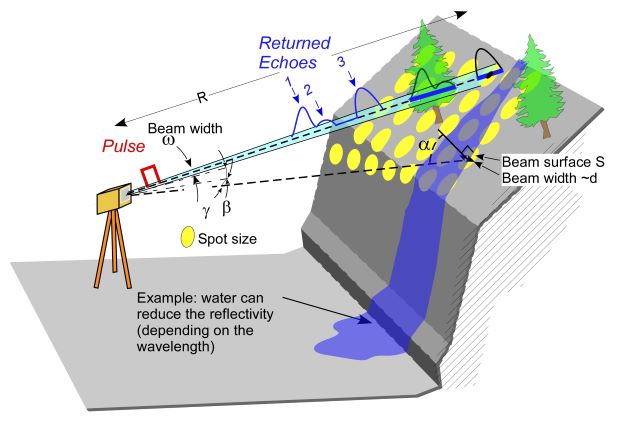
Figure 1: Principles of LiDAR measurement using the example of a TLS. We can observe the different effects of the beam divergence on the illuminated area and multiple echoes (modified from Jaboyedoff et al., 2012).
A short history
The principle of LASERs was established by Einstein (1917). The first functional LASER was designed by Theodor Maiman from the Hughes Research Laboratory in 1960. The first experiment of distance measurement by a range finder or “LiDAR” was performed a few months after construction of the LASER (Brooker, 2009). In the 1970s, LASER techniques were used to measure distance precisely using EDM (electronic distance measuring); the first stand-alone devices coupled with a theodolite (Petrie and Toth, 2018a) that often required a reflector, which is not the case for present-day LiDAR.
The first topographic survey of the Earth’s surface was performed by a LASER altimeter deployed on an airplane, providing measurements with an accuracy greater than 30 cm at 300 m elevation (Miller, 1965). In 1984, a topographic survey along a profile was performed by NASA using an airborne oceanic LiDAR (Krabill et al., 1984). The major issue at this time was the positioning. The appearance of Global Positioning Systems (GPS) allowed workers to acquire topographic transects over the Greenland ice sheet with an accuracy of <20 cm (Krabill et al., 1995). The late 1990s experienced the rapid development of the use and appropriation of ALS (Baltsavias, 1999; Wehr and Lohr, 1999; Carter et al., 2001). For instance, ALS was applied to urban 3D data extraction (Haala and Brenner, 1999) and forest stand research (Naesset, 1997; Means et al., 1999).
The TLS developed slightly more slowly than ALS (Petrie and Toth, 2018b). TLS emerged in the late 1990s for surveying and monitoring structures (Gordon et al., 2001; Lichti et al., 2002). Closed-range TLS appeared slightly earlier (Kanade, 1987). Lichti et al. (2000) tested the capabilities of 3D surveys of TLS on a rock dam. After 2002, the number of publications based on that technology increased drastically (Abellan et al., 2016).
Progressively, TLS devices were coupled with global poisoning satellite systems (GNSS) and inertial measurement units (IMU), aiding the development of mobile LiDAR (Manandhar and Shibasaki, 2001). From 2010, the miniaturization of LiDAR, reduced instrument cost, and drone development made drone-LiDAR available and very powerful for geoscience applications (Lin et al., 2011; Petrie and Toth, 2018a). Furthermore, for a few years, handheld portable LiDAR using IMU has permitted short-range acquisition (10-50 m) by simply walking (ZEB-REVO by geoslam.com) (Figure 2). It may also include a GNSS such as the Pegasus Backpack system (Petrie and Toth, 2018c).
The “boom” of applications for landslide studies mainly began after the year 2000. The first development of slope characterization occurred before 1990 based on LASER-EDM instruments, which were used to monitor rock faces along profiles in mines (Petrie, 1990). One of the first applications of LiDAR was dedicated to the characterization of rock discontinuity orientations and sizes based on TLS (Slob et al., 2002; Kemeny and Post, 2003). The roughness of rock discontinuities was studied by Fardin et al. (2004). ALS hillshade DEMs were used, once sufficiently high-resolution DEMs were available to map and characterize landslides (Carter et al., 2001; Chigira et al., 2004; Haugerud et al., 2003; McKean and Roering, 2004; Ardizzone et al., 2007). Detection of sequences of rockfalls has been performed by calculating the differences between successive TLS PCs (Lim et. al., 2005; Rosser et al., 2005; Collins and Sitar, 2008; Abellan et al., 2010, Williams et al. 2018). Some authors monitored landslide movements and slope evolution based on time series TLS scans (Teza et al., 2007; Collins and Sitar, 2008).
The rich history of LASER scanning has been described in more detail by Shan and Toth (2018), Brooker (2009) and Jaboyedoff et al. (2018).
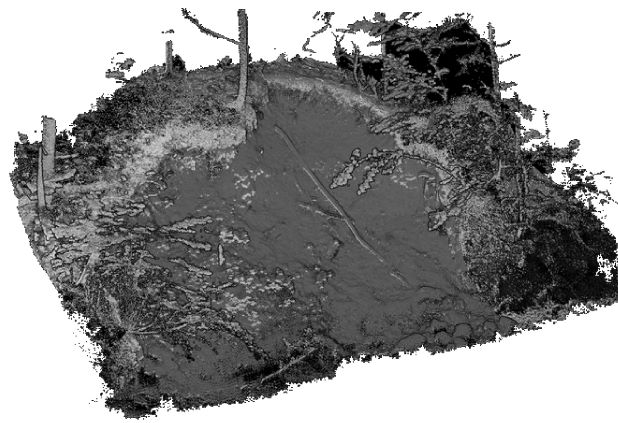
Figure 2: PC of a 5m high landslide (in dark) along a river acquired with a ZEB-REVO LiDAR (geoslam.com). The PC was acquired under forest cover with a density that precludes GNSS positioning. Then an IMU system is used for relative positioning.
Basics of Laser scanners
Lasers and safety
The LiDAR technology is based on a LASER (light amplification by stimulated emission of radiation) with wavelengths from approximately 300 nm to 2000 nm. LASERs are based on electron excitation of specific atoms (often impurities) by lights. The electrons in atoms have specific energy levels that are called E0, E1, E2, and so on. LASERS are able to excite electrons in a metastable energy level from E0 to E1 by transitions from a higher energy state E2, or by simulating another electron with the exact E1 energy level. This leads to the so-called population inversion, i.e., the number of excited electrons exceeds the number of electrons in the ground state E0 ; and the transition from E1 to E0 provides a light with a precise wavelength λ = hc/(E1-E0), where h is Planck’s constant and c the speed of light. The result is a coherent light that is collimated by different techniques. LASER sources mainly include solid-state material, gas, or semiconductors. Notably, LASERs can be dangerous for eyes and skin because of the collimation, coherence and subsequent intensities. The higher the power, the greater the potential injury to eyes and skin for any wavelength of UV visible and infrared light. There are different classes of LASER, with class 1 being the least dangerous and generally safe. Various types of LASERs are used for LiDAR, from class 1 to class 4. The recommendation for the use of LASERs is that even with class 1, eye exposure should be avoided (Petrie and Toth, 2018b).
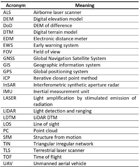
Table 1: Main acronyms used in the text.
LiDAR devices
There are several types of LiDAR. All send LASER pulses or waves, which may have different shapes. The receiver receives the range R from the time of flight (TOF) of the pulse, or by solving R based on signal amplitude modulations inducing frequency modulations. The position relative to the LiDAR is provided by the orientation of the beam, guided by one or two rotating mirrors or/and by the device rotation or motion. The position is either relative to the LiDAR ( β and γ angles) or located (georeferenced) using differential GNSS (DGNSS) coupled with an IMU to obtain the full position and orientation (rotation in all axis) of the device (Figures 1 and 3). Some LiDAR devices are now only equipped with an IMU that provides no georeferenced PCs but allows for working underground or inside buildings.
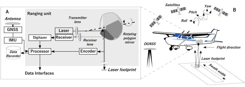
Figure 3: (A) Main hardware components of an ALS RIEGL system (and (B) airborne simple configuration including a navigation system Panel (A): Modified from Petrie and Toth (2018b). Panel (B): Modified from Wehr, A., 2018. LiDAR systems and calibration. In: Shan, J., Toth, C.K. (Eds.), Topographic Laser Ranging and Scanning, second ed. CRC Press, Boca Raton, FL, pp. 1–28
TOF LiDAR
Most long-range LiDARs use TOF (Δt) measurements to obtain the distance (Beraldin et al., 2010):
R=c/n *∆t/2
where c is the speed of the light and n is the index of refraction of the air; n depends on the air temperature, humidity and pressure (and is nearly equal to 1). The LASER sends a pulse (the shape depends on the manufacturer) with a duration of the order of nanoseconds, which is diffused and/or reflected depending on the type of material scanned. The return signal can include several echoes, i.e., TOFs, which are detected by various techniques, such as the maximum of each peak or the exceeding of a predefined threshold; it typically uses a constant fraction detection, i.e., it sets the echo threshold at a given ratio of its maximum amplitude (Beraldin et al., 2010). Most devices provide echoes extracted from the full wave signal without providing the full wave signal itself.
LiDAR using phase measurements
LiDAR instruments with modulation of signal amplitude are mostly used for short-range applications (< 100 m). They can be used in specific situations to monitor movements due to their high accuracy. The distances are provided by solving a set of the following equation (Petrie and Toth, 2018a):
R=0.5 (Mλc+ Δλc)
In the case of amplitude modulation, λc is the wavelength of the measured modulated wave (longer than that of the LASER, which is the carrier wave), M is the integer number of the wavelength, and Δλc is a fraction of the wavelength equivalent to the phase shift Φ (Δλc = λc Φ/2π). This can only be solved if several wavelengths are used (Petrie and Toth, 2018a). Some LASERs allow for frequency modulation, by using a long regular modulation of several milliseconds. The TOF is estimated from the shift of frequencies between the emitted and returned signals. (Brooker, 2009; Beraldin et al., 2010). Another possibility to obtain R from the above equation is to modulate two frequencies in order to reach the conditions for which Δ λ 1 = Δ λ 2= 0 (Brooker, 2009).
LASER scanning based on triangulation
This type of LiDAR can be highly precise, but the range of measured distance does not exceed 5 m. It is based on a triangulation method. The beam of backscattered light is collected by a detector in an aperture distant from the LASER source (Beraldin et al., 2010). The detector is located at a precise and constant distance behind the aperture, providing the angle of the returned beam entering in the aperture. This allows for the determination of the distance and position of the points scanned from the angle of the incident beam and the distance between the LASER source and the detector.
Beam characteristics
A LASER beam is not fully collimated; the minimum divergence ω is given by Wehr (2018):
ω=2.44 λ/D
where D is the aperture diameter. The value is usually provided by the manufacturer based on the shape of the beam. The diameter d of the footprint or illumination spot, perpendicular to the beam, is given by Wehr (2018):
d≈D+ωR or d≈ ωR
which ranges from 30 cm to 2.7 m, assuming R = 1000 m for usual values of w for LiDAR : 0.3 – 2.7 mrad (Wehr, 2018). The power collected Pr by the receiver of area A can be approximately calculated assuming a beam illuminates a Lambertian surface larger than the beam footprint and is perpendicular to it. If ρ is the reflectivity, Ma is the atmospheric transmission, and the transmitted power is PT, then Pr is given by (Baltsavias, 1999):
Pr≈ ρ (M2 Ar)/(π R2 ) PT
For example, assume M = 0.8, ρ = 0.5, R = 1000 m, Ar = π 0.12 = 0.00785 m2 , and PT = 2000 W; then Pr = 8.0 10-10 and PT = 1.60 10-6 W. This can vary depending on the hypothesis about the reflection type. For more details about beam geometry and LiDAR acquisition techniques, please refer to Baltsvias (1999), Wehr and Lohr (1999) and Wehr (2018). In addition, if the illuminated surface is not perpendicular to the beam, then Pr must be replaced by:
P’r ≈ Pr cos ∝
This occurs in the case of a Lambertian diffused reflector where a is the angle between the beam and the normal to the surface, showing that the transmitted power decreases with increasing α (Carrea et al., 2016). Furthermore, an additional geometric factor must be taken into account; when a beam illuminates a surface S obliquely, the size of the footprint increases proportionally to:
S ~ ωR/cos α
This implies that an echo integrates several distances and creates an asymmetry in the returned pulse (Lichti and Skaloud, 2010).
LiDAR uses
Issues
The above brief theoretical background aids in understanding the limitations of the LiDAR techniques. The first problem is working with low-reflectivity surfaces, which drastically decrease the maximum distance that can be detected. This can depend on the surface color and roughness, as dusty surfaces have very low reflectivity. Depending on the wavelength, moisture and ice can also absorb the beam. In our experience, the color of the illuminated area can also marginally affect distance measurements (max. a few mm). The footprint has an impact because the return signal can contain a mix of several contributions, if there are different surfaces with different orientations within the illuminated area or slightly different distances from the LiDAR. If these surfaces are separated by enough distance, the LiDAR will detect several echoes. And if α is sufficiently large; the echo is asymmetrical and influences the intensity and the X, Y, Z point position.
Some less frequent issues can be linked to n the refraction index of the atmosphere. It can change with temperature; which can be linked, for instance, to hot wind ascending along cliffs. Air moisture can also impact n. These variations in n modify the light velocity and can induce beam distortions leading to unprecise X, Y, Z point locations and coordinates. The device itself can also generate problems due to misalignments, moisture in the device, dirty optics, or a decrease in LASER power.
Different LiDAR configurations
Currently, the evolution is so fast in terms of LASER scanning that it is almost impossible to provide a complete up-to-date overview. The acquisition frequency is from 10 kHz to 1 MHz and is not an issue for most applications. The accuracy can be improved to reach millimeter accuracy for static acquisitions by TLS. When using GNSS and IMU for in-motion acquisition (ALS, Drone, Mobile), the results can vary but one can expect a data accuracy of a few centimeters. The choice of tool primarily depends on the acquisition needs, and the environment. For instance, a TLS device can be equipped to function as a mobile LiDAR, which is sufficient for many applications. No recommendations can be made because of the versatility of the systems. Drone –LiDAR and handheld portable LiDAR (Figure 2) will be increasingly used in the near future.
It is important to consider the influence of the acquisition viewpoints used during scanning. (1) Parts of the surface can be hidden by occlusion (Sturzenegger and Stead, 2009; Lato el al., 2010). With a static LiDAR, several scans can be acquired and merged to overcome this issue but drone – LiDAR may solve most of this problem because of its versatility, nearly 360° view and flexibility in the altitude of flight. (2) The point density can also vary greatly depending on the angle of view α. This can bias analyses of the surface orientation such as discontinuities in rock (Sturzenegger and Stead, 2009; Lato el al., 2010). To image in 3D, it is best to be closer to the perpendicular of the surface. As ALS can produce low-density PCs along nearly vertical rock walls.
Filtering
For landslide research, in most of the cases, the last echo is used to generate the point cloud or a DTM. Ocasionally in locations where dense vegetation completely hides the ground, the last pulse is not the ground. For most cases, it is necessary to remove the vegetation echoes from the PC by hand or using automatic or semiautomatic methods. If there are RGB values or infrared attributes for each point, they can be used to discriminate vegetation (Lichti, 2005). Brodu and Lague (2012) have proposed analyses of Eigenvalues of neighboring points to discriminate the vegetation from the more structured points using multiscale criterion. This is implemented in CloudCompare free software (Girardeau-Montaut, 2006) and several other methods exist as well.
Georeferencing and coregistration
Usually, point clouds or DEMs are transformed to obtain an absolute position in a known geographic coordinate system such as Universal Transverse Mercator (UTM). This is performed in several ways. Classically, it was performed using ground control points (GCP), which were used to adjust the position based on least square methods. Since the advent of DGNSS and IMU, GCPs are not necessarily required for most ALS, drone and mobile LiDAR (El-Sheimy, 2018).
A single PC can be georeferenced using GCP acquired using DGNSS. In landslide studies, the absolute position is often not necessary and approximate orientations and horizontality are sufficient because many applications examine the differences between two or more PCs or require only a precision of 1° in orientation. Thus, the second PC is aligned on the first one using fixed references, i.e., parts of the topography that have not changed (i.e., were unaffected by landslide deformation) using the iterative closest point method (ICP), which minimizes the Euclidian distance between the PCs of selected areas (Besl and McKay, 1992; Chen and Medioni, 1992). This procedure is called coregistration. This method is often used to georeference a TLS point cloud on a preexisting DEM even if it has a rather low resolution (25 m).
Coregistration is also frequently used to merge several cloud points to obtain a full view of a topography from different points of view. The point clouds must overlap by at least 20 to 30% to obtain a good result and avoid alignment errors. Georeferencing or coregistration must be checked to compare successive acquisitions or merged scans, where they are overlapped, in order to detect progressive drifts or shifts in the data.
Characterization of landslide
The first tools used are often represented using a hillshade DTM (Boucheny, 2009; Burrough et al., 2015) or slope angle map. Other types of shading such as Eye Dome Lighting (EDL) (Girardeau-Montaut, 2006) or ambient occlusion (Tarini et al., 2006) may improve the visualization of PCs in 3D or DEMs in 2D. Note that some of these tools are implemented in the free software CloudCompare (2018) (Noël et al, 2018). The literature about landslides and LiDAR is now so vast that this chapter only provides a partial view of numerous valuable studies.
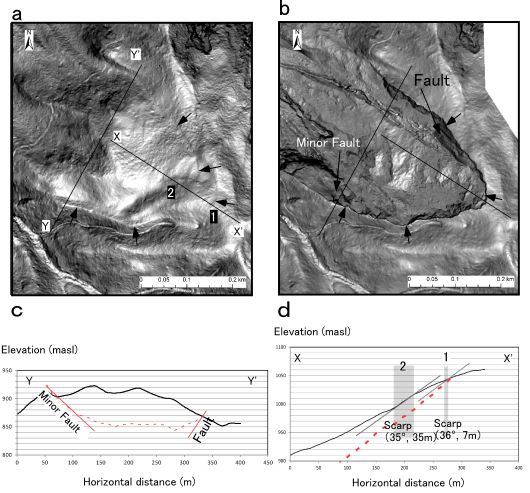
Figure 4: Slope angle map of the pre-event (a) and post-event LDTM (b). (a) Geomorphic features underlined by arrows indicate the limits of the future landslide in (b). (c) and (d) show the cross-sections (located in (a) and (b)): the pre-event topography is shown as continuous black lines and dashed lines indicate the post-event topography. Faults in (a) create lateral limits. (d) Scarps are indicated by thin lines and their outcrops are shown in gray (1 and 2) (From Chigira et al., 2013, with permission).
Mapping
Major contributions of LiDAR techniques for landslide studies were rapidly recognized (Carter et al., 2001; Haugerud et al., 2003; Chigira et al., 2004; Ardizzone et al., 2007). Landside mapping using LiDAR DTM (LDTM) is so widespread that it is impossible to conduct an exhaustive review. However, some points can be emphasized. Ardizzone et al. (2007) compared the results of an inventory based on field visits and aerial photos with an inventory based on LDTM. They showed that the LDTM greatly improved the limits of landslides. Attempts to characterize landslides based on LDTM using indexes such as roughness or the second derivative of the LDTM allowed for discriminating the landslide area (McKean and Roering, 2004), but this method may require too much tuning to be efficient.
Visual inspection of LDTM provides an excellent tool to map landslides. As there is no fixed methodology for such an approach, without a field visit, some geological structures may mimic landslide structures. The most important aspect is the ability to detect the incipient movement of landslides before catastrophic failures. By comparing pre- and post-LDTM, Chigira et al. (2013) showed that the large landslides that occurred during Typhoon Talas in Japan (September 2011) – inducing several causalities – were detectable on the pre-event LDTM. Scarps and depressions were visible before the event (Figure 4). This demonstrates that it is possible to identify the existence of landslide initiation that can be reactivated catastrophically because of significant triggering factors such as earthquakes or heavy rainfall.
Rock structure characterization and rockfall sources
In most cases, rockfall initiations are induced by the presence of unfavorable discontinuity orientations and operate by sliding, toppling or other mechanisms (Hungr et al., 2014). That is why structural analysis of rock faces are of primary importance.
The PC allows workers to visualize the discontinuity sets and identify them using many different approaches. They can be selected manually or by fitting planes automatically (Oppikofer et al., 2009; Sturzenegger and Stead, 2009; Gigli and Casagli 2011; Riquelme et al. 2014). Manual identification can be supported by the COLTOP scheme, which provides a unique color per orientation (Jaboyedoff et al., 2007: Assali et al., 2014). LDTMs have also improved understanding of the impact of structures on large rockslides (Jaboyedoff et al., 2009; Chigira et al., 2013).
Several attempts have been made to automatically compute discontinuity sets (Ferrero et al. 2009; Garcia-Selles et al. 2011; Gigli and Casagli 2011; Assali et al., 2014; Riquelme et al. 2014; Dewez et al. 2016). These methods follow different strategies, and each of them has pros and cons: they work rather well on well-defined structures, can be used for a first approach, and require a verification that the chosen set of parameters provide reliable results.
The data extracted from the structural analysis allows for detecting potential zones of instability or evaluating rockfall susceptibility using kinematic tests on PCs (Matasci et al., 2018) or on LDTM (Günther, 2003; Oppikofer et al., 2009; Jaboyedoff et al., 2012; Loye et al., 2012). A simple way to use PC or LDTM is to determine slope angle thresholds based on expert knowledge (Guzzetti et al., 2003; Frattini et al., 2008). More systematic approaches have been developed by Loye et al. (2009), by decomposing the slope angle histogram, extracted from an LDTM, using one or several Gaussian distributions to obtain the morphological elements. It is typically easy to identify rock walls and find the slope angle threshold above which they represent the majority of the morphology.
Volume estimation
Landslide volume estimation is mainly performed using the difference between two LDTMs within the perimeter of the landslide. The LDTMs must first be coregistered. This is often performed for debris flows when pre- and post-event LDEMs are available (Bull et al., 2010; Bremer and Saas, 2012). If only one LDTM exists, the landslide volume depends on the construction method of the failure surface or the reconstruction of the topography before the event. One method is to use the sloping local base level, which allows for reconstructing a quadratic surface mimicking the topography or the failure surface. This surface is built by an iterative computation within the limits of a landslide (Jaboyedoff et al., 2019).
Rockfall volume estimation is usually performed using two successive PCs that are coregistered to determine the differences. This can be performed in several ways. Grids can be created in the direction perpendicular to the rock face around the failure zone, and the differences in these oblique DEMs can be determined by summing the DEM of difference (DoD) within a given perimeter, or using a threshold value for the difference (Rosser el a. 2007; Loye et al., 2016). Other solutions are to triangulate meshes of PCs, eventually smoothed, and calculate the difference between surfaces (Guerin et al., 2017). Another method uses two PCs and, within a given perimeter, creates a PC of the block. The space in between the selected points can be filled completely by tetrahedrons to obtain the block volume (Carrea et al., 2014).
Several studies describe rockfall activity. The results typically show a power law distribution for the volume (Rosser et al., 2007; Royan et al., 2014; Loye et al., 2016), which is very important for rockfall hazard assessment (Hantz et al., 2003). The errors linked to such evaluations have been detailed in Lane et al. (2003) and Schürch et al. (2011).
Monitoring
Landslide monitoring includes several different strategies that lead to a temporal evolution of maps, distances, and other information. They include simple comparisons of periodic LiDAR acquisitions or real-time monitoring. The simplest approach is the detection of surface changes, which can be performed by a simple closest point method (Girardeau-Montaut, 2006). The real-time monitoring is based on frequent acquisition and fast analysis of distance changes in the LiDAR.
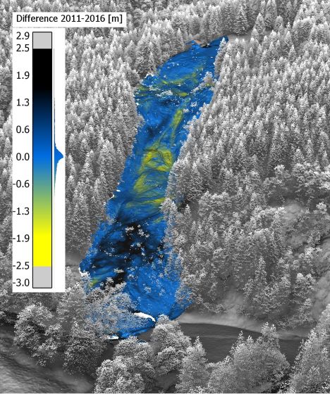
Figure 5: The nonforested area corresponds to the landslide area. This representation includes an LDEM (from the administration of the canton of Vaud, Switzerland) and two TLS acquisitions. The mass movement is estimated using the closest point-to-point distance method. The scale is in meters, positive values show an accumulation and negative values indicate a lowering of the surface. In the central part, material has moved and eroded (up to −2.5 m) and material accumulated at the toe (up to 2 m). HS: headsscarp; MSS; main secondary scarp (modified after Bièvre et al., 2018, with permission).
Surface changes
The DoD allows to estimate the activity of landslides via movements between two different LDTM acquisitions (Burns et al., 2010). This widely used method is fast and allows to rapidly check if acceleration has occurred. It also provides information to understand the deformation and behavior of a landslide.
The activity of the landslide of Pont Bourquin initiated in 2007 near Les Diablerets in the Swiss Prelaps. It is monitored by periodic TLS acquisitions since 2007 and up to now. The comparison of two PCs demonstrates that material is accumulating at its front (Bièvre et al., 2018) (Figure 5). This indicates a mass transfer in the middle of the landslide and an accumulation zone at the bottom.
Multitemporal PCs enable estimations of the rate of cliff retreat from landslides and/or rockfalls along coasts (Rosser et al., 2007; Collins and Sitar, 2008; Lim et al., 2010; Michoud et al., 2015). It is possible to acquire PCs along transportation networks from a vehicle moving faster than 60 km/h to monitor rockfall activity and structures (Lato et al., 2009; Jaboyedoff et al., 2018).
Detailed analysis of rock mass displacements or sequential failures provides information about the failure mechanisms. The monitoring of rock columns in the Åknes rockslide (Norway) by comparison of two PCs demonstrated very small toppling components by extracting the roto-translation matrix (Oppikofer et al., 2009). Similar behavior has been demonstrated in the Dolomite (Italy) (Viero et al., 2010). Abellan et al. (2009) showed that the precision of displacement measurements can be far more accurate than a centimeter and, in our experience, the precision can reach millimeters. Careful monitoring of a rockfall sequence in Yosemite National Park showed that exfoliation joints can propagate by redistribution of stress in a sequence of successive step-by-step failures (Stock et al., 2012). These studies showed how PCs can open new avenues to understand the mechanisms of slope failure (Prokop and Panholzer, 2009).
Potential methods for real-time monitoring
The methods presented in this section can be applied in support of real time monitoring; by recognizing shapes in successive PCs, displacement time series can be generated. It is possible to obtain correspondence between small domains of the PCs and determine the vectors of displacement (Teza et al., 2007). This has also been performed based on the recognition of a target represented by cubes on vegetated landslides (Franz et al., 2016). This has the advantage of providing monitoring that replaces total stations without requiring on-site prism targets. Other monitoring strategies consist of coupling PCs and image pattern recognition methods on associated hillshades (Travelletti et al., 2014; Fey et al., 2015). This is performed using the correspondence between the 2D image and the PC.
Time series of PCs are efficient in quantifying the deformation path leading to rock mass failure based on filtering PCs and measuring the distance between successive acquisitions (Abellan et al., 2010; Royan et al., 2014). Frequent acquisitions and analysis of displacement allowed for forecasting rockfall during the collapse of the eastern flank of the Eiger (Switzerland) (Oppikofer et al., 2008).
Real-time LiDAR monitoring has been developed for mining companies. Using 4D filtering techniques and averaging PCs. Kromer et al. (2017) used this approach to monitor and detect slope movements. Monitoring of the Sechilienne (France) rockslide allowed for following the prefailure displacement of a rock mass (Figure 6). Unfortunately, LiDAR is very sensitive to bad weather, which can restrict the use of such technique.
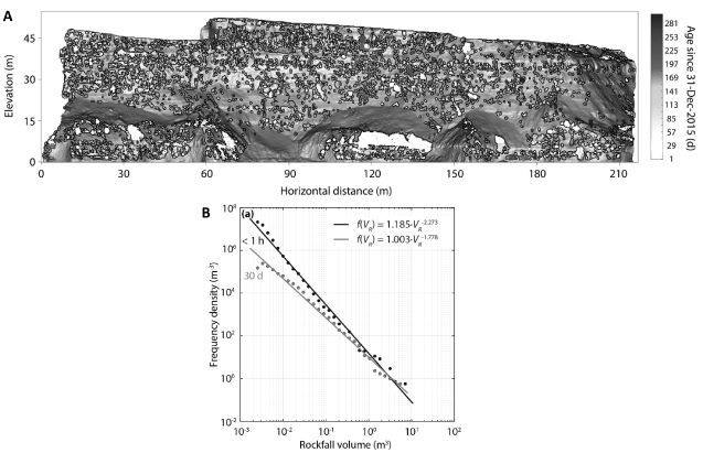
Monitoring a cliff of shales, sandstones and carbonates in the UK every hour for 10 months showed that the contribution of small very frequent detachments of less than 0.1 m3 contributed 98%, instead of 67%, if the interval between acquisitions decreased to less than <1 h instead of 30 days (Williams et al., 2018). This demonstrates that some rockfall events are the result of several smaller events and, if the acquisitions are separated by a longer time lag, the apparent number of rockfalls decreases. This is demonstrated by the steeper slope of the power law distribution of the volumes for frequent acquisitions (Figure 7).
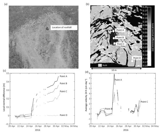
Figure 6: Example of a prefailure deformation of an 80 m3 block, based on PCs acquired every 4 h. A. Block location. B. PC including deformation along the local normal indicated by grayscale. C. Cumulative movement time series of the points A, B and C located on the moving block; Point D is located on an adjacent stable area, the locations are shown on B. D. Velocity for points A, B and C averaged on 24 h. (from Kromer et al., 2017, with permission)
Figure 7: A. Rockfall locations monitored with a time step of less than 1 h for 10 months. The gray scale is the time since December 31st. B. Magnitude–frequency distributions deduced from the above inventory show the differences depending on the acquisition time-step interval, i.e., 1 h or 30 days (modified after Williams et al., 2018).
Modeling based on LDTM
High-precision LDTM has resulted in improvements to landslide models. The first improvement was linked to observations that can be made using PCs or LDTM, which provide details to create complex models of stability (Brideau et al., 2011). The highly detailed topography allows for refining shallow, simple landslide modeling (Dietrich et al., 2001; Baum et al., 2005). The area of high susceptibility surface is reduced compared to coarser DTM because of the high resolution, improving the slope maps and flow accumulation resolution. Using PCs, the susceptibility of rockfall failures can be assessed based on kinematic tests associated with simple geomechanical models. On a rock wall in Yosemite National Park, Matasci et al. (2018) showed that the most active source areas correspond to the high susceptibility zones detected independently on PCs.
The most demonstrative example of improvements is from rockfall modeling. Agliardi and Crosta (2003) showed that the terrain roughness-induced dispersion of the rockfall radically changes rockfall hazard maps. The energy of falling debris is also modified significantly. Recent models take advantage of the fine resolution of the PC instead of the LDTM. The point cloud allows to identify rockfall sources with more precision than the LDTM. This is because the point cloud, unlike the LDTM, can represent vertical or even overhanging faces (Fig. 8). It also has the advantage of including real 3D roughness induced by boulders (Noël et al., 2016). This implies that the rockfall models are closer to “reality”.
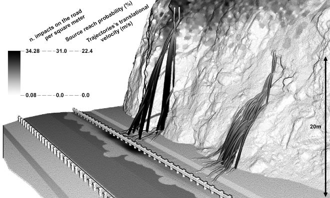
Figure 8: Rockfall model using CP, which can include overhangs. The source area is shown in grayscale, dark gray indicates the probability of reaching the road. The number of impacts per square meter reaching the road is indicated on the road in grayscale. Some block trajectories are indicated, with their velocities. (Modified after Noël et al., 2016).
Discussion and perspectives
As demonstrated earlier, LiDAR has significantly impacted landslide research and practitioners. Although LiDAR acquisition is more expensive than photogrammetric methods, such as structure from motion (SfM), LiDAR has major advantages that often justify its use. It is especially efficient for vegetated areas (Figure 9) and, because LiDAR systems include the georeferencing in most configurations, these methods can be complementary. The applications listed above depend on the distance of acquisition and georeferencing methods, so the level of accuracy and precision can be very high, from millimeters to a few centimeters, and no improvements are needed for standard landslide and geomorphic studies. Notably, the monitoring of landslide movements will be enhanced by improvements in accuracy and precision of point cloud data to understand processes and improve early warning systems (EWS).
The applications shown here may be used by landslide researchers and practitioners as soon as LiDAR PCs or LDTMs are available. This adds incredible value to landslide studies, but such data is best used in combination with field investigations. LiDAR data provide guidance for field investigations and valuable information that cannot be extracted from the field; that is why it is recommended to combine approaches. As shown earlier, LiDAR has improved rockfall, debris flow, landslide, and rockslide characterization, which are important for hazard assessment and risk management.
From a more general perspective, the integration of data from many origins is often the base of any study, for which LiDAR-derived products are strong basic data, particularly for geographic information systems (GIS). The combination of LiDAR and SfM PCs can be an excellent compromise to complete TLS data with SfM acquired by drones or ALS data with SfM data from vertical rock faces. In addition, such mixed documents are very important for communication (Figure 9), which is becoming increasingly important for risk management.
There is potential for development using the information contained in PCs of landslides. For rock mass characterization, there is a wide scope for new and innovativeresearch. For instance, automated characterization of discontinuities is not completely explored (Riquelme et al., 2015). In addition, there are theoretical issues to resolve such as: how to define discontinuity spacing and trace lengths using a PC coupled with images? For landslides, the extraction of potential failure surfaces based on the geomorphic characteristics must be investigated. Based on monitoring using multi-temporal PCs or LDTMs, there is room to develop automatic 3D shape tracking for landslide deformations; a few methods are available but are not necessarily applicable to any type of movement.
Characterization of landslides using LiDAR, DTMs, and PCs remains challenging because, at present, there are gaps in our understanding of how to compute the strain at the surface of landslides, although some studies are available (Teza et al., 2008; Travelletti et al., 2014). Landslide modeling must exploit the full resolution of PCs or LDTMs, with the exception of rockfall modeling, which has already taken advantage of the high resolution.
There will likely be improvements in LiDAR accuracy, precision and acquisition duration in the upcoming years. There are now several types of LiDAR such as TLS, ALS, Mobile LiDAR, LiDAR mounted on drones (Figure 10) and handheld systems. The link with GNSS, IMU and RGB images will be improved and generalized. These advances depend on the development of LiDAR for autonomous cars (Bimbraw, 2015), as the market is so large. This indicates that development and prices will decrease drastically but may not affect long-range devices. The last improvement will come from satellites, as there is no LDTM over the whole earth. A possible first step is the recently launched ICESat-2 satellite (September 2018), designed to monitor the Greenland icecap and provide data for other regions (https://icesat-2.gsfc.nasa.gov/), which will be valuable for regions that lack good DEMs.
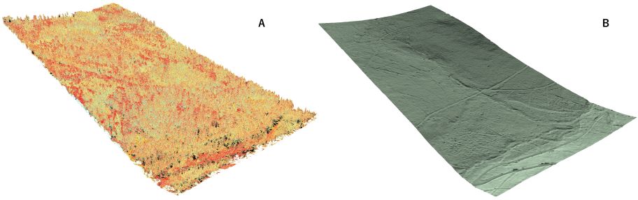
Figure 9: (A) A PC with color intensity depending on reflectance and (B) LDTM after PC treatment. The data were acquired from a drone Ricopter by RIEGL with LiDAR VUX-1. Point density of 100 pts m-1 (Images kindly provided RIEGL).
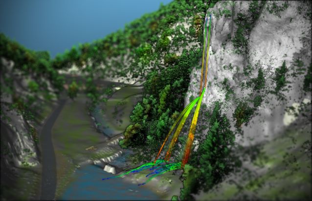
Figure 10: Example of rockfall modeling included in an artificially colorized PC, which can be used for communication to public. This image merges 3 types of data, TLS, SfM and ALS for georeferencing, and was produced using CloudCompare (2018) (From Noël et al. (2018) with permission).
Acknowledgements
We thank the risk group of the Institute of Earth Sciences of the University of Lausanne for the discussion and are especially grateful to Martin Franz, François Noël and Jérémie Voumard who provided us new versions and modified figures. We also thank the RIEGL Company for providing drone LiDAR images. The English language of this manuscript was edited by American Journal Experts, we thank them for their support. We are thankful to Professor Simon Mudd for his fruitful comments on this chapter.
References
Abellán, A., Jaboyedoff, M., Oppikofer, T., and Vilaplana, J. M. 2009. Detection of millimetric deformation using a terrestrial laser scanner: Experiment and application to a rockfall event. Nat. Hazards Earth Syst. Sci., 9, 365–372.
Abellan A,., Vilaplana, J. M., Calvet, J., Blanchard, J., 2010. Detection and spatial prediction of rockfalls by means of terrestrial laser scanning modelling. Geomorphology, 119, 162–171.
Abellán, A., Jaboyedoff, M., Oppikofer, T., Rosser, N. J., Lim, M., Lato, M., 2014. State of science: Terrestrial laser scanner on rock slopes instabilities. Earth Surf. Proc. Landforms, 39, 1, 80–97. DOI: 10.1002/esp.3493.
bellan, A., Derron, M-H., Jaboyedoff, M., 2016. “Use of 3D Point Clouds in Geohazards” Special Issue: Current Challenges and Future Trends. Remote Sensing 8, 130. DOI: 10.3390/rs8020130
Agliardi, F., Crosta, G. B., 2003. High resolution three-dimensional numerical modelling of rockfalls. Int. J. Rock Mech. Min. Sci., 40, 455–471. DOI: 10.1016/S1365-1609(03)00021-2.
Ardizzone, F., Cardinali, M., Galli, M., 2007. Identification and mapping of recent rainfall-induced landslides using elevation data collected by airborne LiDAR. Nat. Hazards Earth Syst. Sci., 7, 637–650.
Assali, P., Grussenmeyer, P., Villemin, T., Pollet, N., Viguier, F., 2014. Surveying and modeling of rock discontinuities by terrestrial laser scanning and photogrammetry: Semiautomatic approaches for linear outcrop inspection, Journal of Structural Geology, 66, 102- 114.
Baltsavias, E.P., 1999. Airborne laser scanning: Basic relations and formulas. ISPRS J. Photogramm. Remote Sens., 54, 199–214.
Baum, R.L., Coe, J.A., Godt, J.W., Harp, E.L., Reid, M.E., Savage, W.Z., Schulz, W.H., Brien, D.L., Chleborad, A.F., McKenna, J.P., Michael, J.A., 2005. Regional landslide-hazard assessment for Seattle, Washington, USA. Landslides 2 (4), 266–279.
Beraldin, J.-A., Blais, F., and Lohr, U., 2010. Laser scanning technology. In Airborne and Terrestrial Laser Scanning, Vosselman, G., and Maas, H.-G., eds. Dunbeath, Scotland: Whittles Publishing, 1–42.
Besl, P., McKay, N., 1992. A method for registration of 3-D shapes. IEEE Trans. Pattern Anal. Mach. Intell., 14, 239–256.
Bièvre, G., Franz, M., Larose, E., Carrière, S., Jongmans, D., Jaboyedoff, M., 2018. Influence of environmental parameters on the seismic velocity changes in a clayey mudflow (Pont-Bourquin Landslide, Switzerland). Eng. Geo., 245, 248-257. doi: doi.org/10.1016/j.enggeo.2018.08.013
Bimbraw K. (2015). Autonomous Cars: Past, Present and Future – A Review of the Developments in the Last Century, the Present Scenario and the Expected Future of Autonomous Vehicle Technology.In Proceedings of the 12th International Conference on Informatics in Control, Automation and Robotics – Volume 1: ICINCO, ISBN 978-989-758-122-9, pages 191-198. DOI: 10.5220/0005540501910198
Boucheny, C., 2009. Visualisation scientifique interactive de grands volumes de données : pour une approche perceptive. Université Joseph Fourier.
Bremer, M., Sass, O., 2012. Combining airborne and terrestrial laser scanning for quantifying erosion and deposition by a debris flow event. Geomorphology, 138(1), 49–60.
Brideau, M. A., Pedrazzini, A., Stead, D., Froese, C., Jaboyedoff, J., van Zeyl, D., 2011. Three-dimensional slope stability analysis of South Peak, Crowsnest Pass, Alberta, Canada. Landslides, 8, 139–158. DOI: 10.1007/s10346-010-0242-8.
Brodu, N., and Lague, D., 2012. 3D terrestrial LiDAR data classification of complex natural scenes using a multi-scale dimensionality criterion: Applications in geomorphology. ISPRS J. Photogramm. Remote Sens., 68, 121–134.
Brooker, G., 2009. Introduction to sensing. In Introduction to Sensors for Ranging and Imaging. Raleigh, NC: The Institution of Engineering and Technology, 743p.
Bull, J. M., Miller, H., Gravley, D. M., Costello, D., Hikuroa, D. C. H., and Dix, J. K., 2010. Assessing debris flows using LiDAR differencing: 18 May 2005 Matata event, New Zealand. Geomorphology, 124, 75–84.
Burns, W. J., Coe, J. A., Kaya, B. S., Ma, L., 2010. Analysis of elevation changes detected from multi-temporal LiDAR surveys in forested landslide terrain in western Oregon. Environ. Eng. Geosci., 16(4), 315–341.
Burrough, P. A., McDonnell, R. A., Lloyd, C. D., 2015. Principles of geographical information systems (Third Ed.). Oxford University Press.
Carrea, D., Abellán A., Derron, M.-H., Jaboyedoff M., 2014. Automatic Rockfalls Volume Estimation Based on Terrestrial Laser Scanning Data. In: G. Lollino et al. (eds.), Engineering Geology for Society and Territory – Vol. 2, Springer, DOI: 10.1007/978-3-319-09057-3_68, 325-328.
Carrea. D., Abellan. A., Humair. F., Matasci. B., Derron. M.-H., Jaboyedoff. M., 2016. Correction of terrestrial LiDAR intensity channel using Oren–Nayar reflectance model: An application to lithological differentiation. ISPRS Journal of Photogrammetry and Remote Sensing: 113, 17–29.
Carter, W., Shrestha, R., Tuell, G., Bloomquist, D., Sartori, M., 2001. Airborne laser swath mapping shines new light on earth’s topography. EOS, 82(46), 549–564.
Chen, Y., Medioni, G., 1992. Object modelling by registration of multiple range images. Image Vis. Comput., 10, 145–155.
Chigira, M., Duan, F., Yagi, H., Furuya, F., 2004. Using an airborne laser scanner for the identification of shallow landslides and susceptibility assessment in an area of ignimbrite overlain by permeable pyroclastics. Landslides, 1, 203–209.
Chigira, M., Tsou, C.-Y., Matsushi, Y., Hiraishi, N., Matsuzawa, M., 2013. Topographic precursors and geological structures of deep-seated catastrophic landslides caused by Typhoon Talas. Geomorphology 201, 479-493.
CloudCompare, 2018. CloudCompare (version 2.9.1) [GPL software], Retrieved from https://www.cloudcompare.org/
Collins, B., Sitar, N., 2008. Processes of coastal bluff erosion in weakly lithified sands, Pacifica, California, USA. Geomorphology, 97, 483–501.
Dewez, T. J. B., Girardeau-Montaut, D., Allanic, C., Rohmer, J., 2016. Facets : a cloudcompare plugin to extract geological planes from unstructured 3d point clouds, Int. Arch. Photogramm. Remote Sens. Spatial Inf. Sci., XLI-B5, 799-804, https://doi.org/10.5194/isprs-archives-XLI-B5-799-2016.
Dietrich, W. E., Bellugi, D., , Real de Asua, R., 2001. Validation of the shallow landslide model, SHALSTAB, for forest management. In Land Use and Watersheds: Human Influence on Hydrology and Geomorphology in Urban and Forest Areas, Wigmosta, M. S., and Burges, S. J., eds. Water Science and Application, vol. 2. Hoboken, NJ: Wiley, 195–227.
Einstein, A., 1917. The Quantum Theory of Radiation. Phys. Z. 18, 121 (1917.
El-Sheimy, N., 2018. Georeferencing Component of LiDAR Systems. In Topographic Laser Ranging and Scanning (2nd Ed.), Shan, J., and Toth, C. K., eds. Boca Raton, FL: CRC Press, 221-238.
Fardin, N., Feng, Q., , Stephansson, O., 2004. Application of a new in situ 3D laser scanner to study the scale effect on the rock joint surface roughness. Int. J. Rock Mech. Min. Sci., 41, 329–335.
Ferrero, A. M., Forlani, G., Roncella, R., Voyat, H. I., 2009. Advanced geostructural survey methods applied to rock mass characterization. Rock Mech. Rock Eng., 42(1), 631–665. DOI: 10.1007/s00603 -008-0010-4.
Fey, C., Rutzinger, M., Wichmann, V., Prager, C., Bremer, M., Zangerl, C., 2015. Deriving 3D displacement vectors from multi-temporal airborne laser scanning data for landslide activity analyses. GIScience & Remote Sensing, 52(4), 437–461.
Franz, M., Carrea, D., Abellán, A, Derron, M-H, Jaboyedoff, M. 2016. Use of targets to track 3D displacements in highly vegetated areas affected by landslides. Landslides, 13: 821–831. DOI 10.1007/s10346-016-0685-7.
Frattini P, Crosta G, Carrara A, Agliardi F, 2008. Assessment of rockfall susceptibility by integrating statistical and physically-based approaches. Geomorphology 94:419-437
Garcia-Selles, D., Falivene, O., Arbues, P., Gratacos, O., Tavani, S., Munoz, J. A., 2011. Supervised identification and reconstruction of near-planar geological surfaces from terrestrial laser scanning. Comput. Geosci., 37, 1584–1594. DOI: 10.1016/j.cageo.2011.03.007.
Gigli, G., Casagli, N., 2011. Semi-automatic extraction of rock mass structural data from high resolution LiDAR point clouds. Int. J. Rock Mech. Min. Sci., 48, 187–198.
Girardeau-Montaut, D., 2006. Détection de changement sur des données géométriques tridimensionnelles. Doctorat Traitement du Signal et des Images, TSI/TII, ENST. https://tel.archives-ouvertes.fr /pastel-00001745/.
Glenn, N. F., Streutker, D. R., Chadwick, D. J., Thackray, G. D., Dorsch, S. J., 2006. Analysis of LiDAR derived topographic information for characterizing and differentiating landslide morphology and activity. Geomorphology, 73(1–2), 131–148.
Gordon, S., Litchi, D., Stewart, M., 2001. Application of a high-resolution, ground-based laser scanner for deformation measurements. In New Techniques in Monitoring Surveys I, Proceedings of the 10th FIG International Symposium on Deformation Measurements, Orange, California, 23–32, 19–22 March 2001.
Guerin, A., Abellán, A., Matasci, B., Jaboyedoff, M., Derron, M.-H., and Ravanel, L, 2017. Brief communication: 3-D reconstruction of a collapsed rock pillar from Web-retrieved images and terrestrial lidar data – the 2005 event of the west face of the Drus (Mont Blanc massif), Nat. Hazards Earth Syst. Sci., 17, 1207-1220, https://doi.org/10.5194/nhess-17-1207-2017, 2017.
Günther, A., 2003. Slopemap: programs for automated mapping of geometrical and kinematical properties of hard rock hill slopes. Computer & Geosciences 29(7):865-875
Guzzetti, F., Reichenbach, P., Wieczorek, G. F., 2003. Rockfall hazard and risk assessment in the Yosemite Valley, California, USA. Nat. Hazards Earth Syst. Sci., 3, 491–503.
Haala, N., and Brenner, C. 1999. Extraction of buildings and trees in urban environments. ISPRS J. Photogramm. Remote Sens., 54, 130–137.
Hantz, D., Vengeon, J. M., Dussauge-Peisser, C., 2003. An historical, geomechanical and probabilistic approach to rock-fall hazard assessment, Nat. Hazards Earth Syst. Sci., 3, 693-701, https://doi.org/10.5194/nhess-3-693-2003.
Haugerud, R. A., Harding, D. J., Johnson, S. Y., Harless, J. L., Weaver, C. S., Sherrod, B. L., 2003. Highresolution lidar topography of the Puget Lowland, Washington—A Bonanza for earth science. GSA Today, 13, 4–10.
Hungr, O., Leroueil, S., Picarelli, L., 2014. The Varnes classification of landslide types, anupdate. Landslides 11, 167–194. https://doi.org/10.1007/s10346-013-0436-y.
Jaboyedoff, M., Metzger, R., Oppikofer, T., Couture, R., Derron, M. H., Locat, J., Turmel, D., 2007. New insight techniques to analyze rock-slope relief using DEM and 3D-imaging cloud points: COLTOP-3D software. In Rock mechanics: Meeting Society’s Challenges and demands, Vol. 1, pp. 61–68, Vancouver, BC, Canada.
Jaboyedoff, M., Couture, R., Locat, P., 2009. Structural analysis of Turtle Mountain (Alberta) using digital elevation model: Toward a progressive failure. Geomorphology, 103, 5–16. DOI: 10.106/j.geomorph .2008. 14.012.
Jaboyedoff, M., Oppikofer, T., Abellan, A., Derron, M.-H., Loye, A., Metzger, R., Pedrazzini, A., 2012. Use of LiDAR in landslide investigations: A review. Nat. Hazards, 61, 5–28. DOI: 10.1007/s11069 -010-9634-2.
Jaboyedoff M., Abellán A., Carrea D, Derron M.-H., Matasci B. Michoud C., 2018. LiDAR Use for Mapping and Monitoring of Landslides. In Encyclopaedia of Natural Hazards, Singh R., Bartlett D. (Eds.). Taylor & Francis, p. 397-420.
Jaboyedoff, M., Chigira, M., Arai, N., Derron, M.-H., Rudaz, B., Tsou, C.-Y. (2019). Testing a failure surface prediction and deposit reconstruction method for a landslide cluster that occurred during Typhoon Talas (Japan), Earth Surf. Dynam. Discuss., https://doi.org/10.5194/esurf-2018-61.
Kanade T. 1987. Three-dimensional machine vision. Kluwer academic publisher. 609 p.
Kemeny, J., Post, R., 2003. Estimating three-dimensional rock discontinuity orientation from digital images of fracture traces. Comput. Geosci., 29, 65–77.
Krabill, W. B., Collins, J. G., Link, L. E., Swift, R. N., Butler, M. L. 1984. Airborne laser topographic mapping results. Photogramm. Eng. Remote Sens., 50, 685–694.
Krabill, W. B., Thomas, R. H., Martin, C. F., Swift, R. N., Frederick, E. B. 1995. Accuracy of airborne laser altimetry over Greenland ice sheet. Int. J. Remote Sens., 16, 1211–1222.
Kromer, R. A., Abellán, A., Hutchinson, D. J., Lato, M., Edwards, T., Jaboyedoff, M., 2015. A 4D filtering and calibration technique for small-scale point cloud change detection with a terrestrial laser scanner. Remote Sensing, 7(10), 13029–13052.
Kromer, R. A., Abellán, A., Hutchinson, D. J., Lato, M., Chanut, M.-A., Dubois, L., Jaboyedoff, M. 2017. Automated terrestrial laser scanning with near-real-time change detection – monitoring of the Séchilienne landslide, Earth Surf. Dynam., 5, 293-310, https://doi.org/10.5194/esurf-5-293-2017.
Lane, S. N., Westaway, R. M., and Murray Hicks, D., 2003. Estimation of erosion and deposition volumes in a large, gravel-bed, braided river using sysnotpic remoe sensing, Earth Surf. Proc. Land., 28, 249–271.
Lato, M., Hutchinson, J., Diederichs, M., Ball, D., Harrap, R., 2009. Engineering monitoring of rockfall hazards along transportation corridors: Using mobile terrestrial LiDAR. Nat. Hazards Earth Syst. Sci., 9, 935–946.
Lato, M. J., Diederichs, M. S., Hutchinson, D. J., 2010. Bias correction for view-limited LiDAR scanning of rock outcrops for structural characterization. Rock Mech. Rock Eng., 43(5), 615–628. DOI: 10.1007 /s00603-010-0086-5.
Lichti, D, Stewart, M, Tsakiri, M, Snow, A., 2000. Benchmark Tests on a Three-dimensional Laser Scanning System. Geomatics Research Australasia 72:1-24
Lichti, D., Gordon, S., Stewart, M., 2002. Ground-based laser scanners: Operation, systems and applications. Geomatica, 56(1), 21–33.
Lichti, D.D., 2005. Spectral filtering and classification of terrestrial laser scanner point clouds. Photogramm. Rec., 20, 218–240.
Lichti, D. D., Skaloud, J., 2010. Registration and calibration. In Airborne and Terrestrial Laser Scanning, Vosselman, G., and Maas, H.-G., eds. Caithness, UK: Whittles Publishing, 83–133.
Lim, M., Petley, D. N., Rosser, N. J., Allison, R. J., Long, A. J., Pybus, D., 2005. Combined digital photogrammetry and time-of-flight laser scanning for monitoring cliff evolution. Photogramm. Rec., 20(1), 109–129.
Lim, M., Rosser, N.J., Allison, R.J., Petley, D.N., 2010. Erosional processes in the hard rock coastal cliffs at Staithes, North Yorkshire. Geomorphology, 114, 12–21.
Lin, Y., Hyyppa, J., Jaakkola, A., 2011. Mini-UAV-borne LiDAR for fine-scale mapping. IEEE Geosci. Remote S., 8(3), 426–430.
Loye, A., Pedrazzini, A., Theules, J., Jaboyedoff, M., Liébault, F., & Metzger, R., 2012. Influence of bedrock structures on the spatial pattern of erosional landforms in small alpine catchments. ESPL, 37, 1407-1423.
Loye, A., Jaboyedoff, M., Pedrazzini, A., 2009. Identification of potential rockfall source areas at regional scale using a DEM-based quantitative geomorphometric analysis. Nat. Hazards Earth Syst. Sci., 9, 1643–1653. DOI: 10.5194/nhess-9-1643-2009.
Loye A., Jaboyedoff, M., Theule, J., Liébault, F., 2016. Headwater sediment dynamics in a debris flow catchment constrained by high-resolution topographic surveys. Earth Surf. Dynam. 4, 489–513.
Manandhar, D., Shibasaki, R., 2001. Vehicle-borne laser mapping system (VLMS) for 3-D GIS, paper presented at IGARSS 2001. Scanning the Present and Resolving the Future. Proceedings. IEEE 2001 International Geoscience and Remote Sensing Symposium (Cat. No.01CH37217), 9-13 July 2001.
Matasci, B., Stock, G.M., Jaboyedoff, M., Carrea, D., Collins, B.D., Guérin, A., Matasci, G., Ravanel, L., 2018. Assessing rockfall susceptibility in steep and overhanging slopes using three-dimensional analysis of failure mechanisms. Landslides: 15:859–878. DOI 10.1007/s10346-017-0911-y
McKean, J., Roering J. J., 2004. Landslide detection and surface morphology mapping with airborne laser altimetry. Geomorphology, 57, 331–351.
Means, J.E., Acker, S.A., Harding, D.J., Blair, J.B., Lefsky, M.A., Cohen W.B., Harmon, M.E., McKee, W.A., 1999. Use of Large-Footprint Scanning Airborne Lidar To Estimate Forest Stand Characteristics in the Western Cascades of Oregon, Remote Sensing of Environment, 67(3), 298-308, doi:https://doi.org/10.1016/S0034-4257(98)00091-1.
Michoud, C., Carrea, D., Costa, S., Derron, M., Jaboyedoff, M., Delacourt, C., Maquaire, O., Letortu, P., Davidson, R., 2015. Landslide detection and monitoring capability of boat-based mobile laser scanning along Dieppe coastal cliffs, Normandy. Landslides, 12(2), 403–418.
Miller, B., 1965. Laser altimeter may aid photo mapping. Aviat. Week Space Technol., 88, 60–64.
Næsset, E., 1997. Determination of mean tree height of forest stands using airborne laser scanner data. ISPRS Journal of Photogrammetry and Remote Sensing, 52, 49–56.
Noël, F., Cloutier, C., Turmel, D., Locat, J., 2016. Using point clouds as topography input for 3D rockfall modeling. In Landslides and Engineered Slopes. Experience, Theory and Practice, Napoli, Italy: CRC Press, pp. 1531–1535.
Noël, N., Derron, M.-H., Jaboyedoff, M., Cloutier, C. and Locat, J., 2018. Optimizing the use of 3D point clouds data for a better analysis and communication of 3D results. 3rd Virtual Geoscience Conference (VGC), 2p.
Oppikofer, T., Jaboyedoff, M., Keusen, H. R., 2008. Collapse at the eastern Eiger flank in the Swiss Alps. Nat. Geosci., 1, 531–535.
Oppikofer, T., Jaboyedoff, M., Blikra, L., Derron, M.-H., Metzger, R., 2009. Characterization and monitoring of the Aknes rockslide using terrestrial laser scanning. Nat. Hazards Earth Syst. Sci., 9, 1003–1019.
Petrie, G., 1990. Laser-based surveying instrumentation and methods. In Engineering Surveying Technology, Kennie, T. J. M., and Petrie, G., eds. London: Halsted Press, 48–83.
Petrie, G., Toth, C., 2018a. Introduction to laser ranging, profiling, and scanning. In Topographic Laser Ranging and Scanning (2nd Ed.), Shan, J., and Toth, C.K., eds. Boca Raton, FL: CRC Press, 1–28.
Petrie, G., Toth, C., 2018b. Airborne and spaceborne laser profilers and scanners. In Topographic Laser Ranging and Scanning (2nd Ed.), Shan, J., and Toth, C. K., eds. Boca Raton, FL: CRC Press, 89–157.
Petrie, G., Toth, C., 2018c. Terrestrial Laser Scanners. In Topographic Laser Ranging and Scanning (2nd Ed.), Shan, J., and Toth, C.K., eds. Boca Raton, FL: CRC Press, 29-88.
Pradhan B. (Ed.) 2017. Laser Scanning Applications in Landslide Assessment. Springer. 359 p.
Prokop, A., Panholzer, H., 2009. Assessing the capability of terrestrial laser scanning for monitoring slow moving landslides. Nat. Hazards Earth Syst. Sci., 9, 1921–1928.
Riquelme, A., Abellan, A., Tomás, R., and Jaboyedoff, M., 2014. A new approach for semi-automatic rock mass joints recognition from 3D point clouds. Comput. Geosci., 68(0), 38–52. DOI: 10.1016/j.cageo.2014 .03.014.
Riquelme, A., Abellan, A., Tomás, R., 2015. Discontinuity spacing analysis in rock masses using 3D point clouds. Eng. Geol. 195, 185–195. DOI:10.1016/j.enggeo.2015.06.009.
Rosser, N. J., Petley, D. N., Lim, M., Dunning, S. A., Allison, R. J., 2005. Terrestrial laser scanning for monitoring the process of hard rock coastal cliff erosion. Q. J. Eng. Geol. Hydrogeol., 38, 363–375.
Rosser, N. J., Lim, N., Petley, D. N., Dunning, S., Allison, R. J., 2007. Patterns of precursory rockfall prior to slope failure. J. Geophys. Res., 112(F4), F04014, 14 p, doi:10.1029/2006JF000642.
Royan, M. J., Abellán, A., Jaboyedoff, M., Vilaplana, J. M., Calvet, J., 2013. Spatio-temporal analysis of rockfall pre-failure deformation using terrestrial LiDAR. Landslides, 11, 697–709. DOI: 10.1007/s10346 -013-0442-0.
SafeLand Deliverable 4.1, 2010. Michoud, C., Abella´n, A., Derron, M.-H., Jaboyedoff, M. (Eds.), Review of Techniques for Landslide Detection, Fast Characterization, Rapid Mapping and Long-Term Monitoring. Edited for the SafeLand European project by https://www.ngi.no/eng/Projects/SafeLand. Schürch, P., Densmore, A., Rosse, N., Lim, M., McArdell, B. W., 2011. Detection of surface change in complex topography using terrestrial laser scanning: Application to the Illgraben debris-flow channel. Earth Surf. Proc. Landforms, 36, 1847–1859.
Shan J., Toth, K., 2018. Topographic Laser Ranging and Scanning: Principles and Processing. Boca Raton, FL: CRC Press, Taylor & Francis Group.
Slob, S., Hack, R., Keith, T., 2002. An approach to automate discontinuity measurements of rock faces using laser scanning techniques. In Proceedings of the International Symposium on Rock Engineering for Mountainous Regions—Eurock 2002, Funchal, Portugal, 25–28 November, 87–94.
Stock, G. M., Martel, S. J., Collins, B. D., Harp, E. L., 2012. Progressive failure of sheeted rock slopes: The 2009–2010 Rhombus Wall rock falls in Yosemite Valley, California, USA. Earth Surf. Proc. Landforms, 37, 546–561.
Sturzenegger, M., and Stead, D., 2009. Quantifying discontinuity orientation and persistence on high mountain rock slopes and large landslides using terrestrial remote sensing techniques. Nat. Hazards Earth Syst. Sci., 9, 267–287.
Tarini, M., Cignoni, P., Montani, C., 2006. Ambient Occlusion and Edge Cueing to Enhance Real Time Molecular Visualization. IEEE Transactions on Visualization and Computer Graphics, 12(5).
Teza, G., Galgaro, A., Zaltron, N., Genevois. R., 2007. Terrestrial laser scanner to detect landslide displacement fields: A new approach. Int. J. Remote Sens., 28(16), 3425–3446.
Travelletti, J., J.-P. Malet, C. Delacourt 2014. Image-based correlation of Laser Scanning point cloud time series for landslide monitoring, International Journal of Applied Earth Observation and Geoinformation, 32, 1-18, doi:https://doi.org/10.1016/j.jag.2014.03.022.
Viero A., Teza T., Massironi M., Jaboyedoff M., Galgaro A. 2010. Laser scanning-based recognition of rotational movements on a deep seated gravitational instability: The Cinque Torri case (North-Eastern Italian Alps). Geomorphology, 122, 191-204.
Vosselman, G., Maas, H., 2010. Airborne and Terrestrial Laser Scanning. Boca Raton, FL: CRC Press. 318 p.
Wehr A. 2018. LiDAR Systems and Calibration. In Topographic Laser Ranging and Scanning (2nd Ed.), Shan, J., and Toth, C.K., eds. Boca Raton, FL: CRC Press, 1–28.
Wehr, A., Lohr, U., 1999. Airborne laser scanning—An introduction and overview. ISPRS J. Photogramm. Remote Sens., 54, 68–82.
Williams, J. G., Rosser, N. J., Hardy, R. J., Brain, M. J., Afana, A. A., 2018. Optimising 4D approaches to surface change detection: Improving understanding of rockfall magnitude-frequency, Earth Surf. Dynam. Discuss., https://doi.org/10.5194/esurf-2017-43.
Further reading
Zwally, H. J., Schutz, B., Abdalati, W., Abshire, J., Bentley, C., Brenner, A., Bufton, J. et al., 2002. ICESat’s laser measurements of polar ice, atmosphere, ocean, and land. J. Geodyn., 34, 405–445.