Michel Jaboyedoff1, Pascal Horton1, Marc-Henri Derron1, Céline Longchamp1, Clément Michoud1
1University of Lausanne, Lausanne, Switzerland
Jaboyedoff M., Horton P., Derron MH., Longchamp C., Michoud C. (2013) Monitoring Natural Hazards. In: Bobrowsky P.T. (eds) Encyclopedia of Natural Hazards. Encyclopedia of Earth Sciences Series. Springer, Dordrecht. DOI: 10.1007/978-1-4020-4399-4_354 and PDF
Synonyms
Surveillance, watching, observation
Definition
The verb “to monitor” comes from the Latin “monere” which means to warn. In geosciences, it means to watch carefully a hazardous situation and to observe its evolution and changes over a period of time. It is also used to define the activity of a device that measures periodically or continuously sensitive states and specific parameters.
Introduction
Hazard monitoring is based on the acquisition and the interpretation of a signal indicating changes in behaviour or properties of a hazardous phenomenon or the occurrence of events. This ranges from acquiring basic meteorological data to advanced ground movement measurements. Hazards monitoring began some time ago, when the Babylonians first tried to forecast weather. When Aristotle wrote his treatise Meteorologica, the Chinese were also aware of weather observations (NASA, 2012a). Pliny the Elder studied in detail the eruption of the Vesuvius in August 79 AD, providing one of the first scientific observations of a natural catastrophe. Presently, the evolution and the precision of monitoring are closely linked to the development of new technologies. A very interesting example highlighting the importance of technological development is provided by hurricane statistics. The number of hurricanes had often been underestimated because of the lack of information prior to the appearance of satellite imagery: many hurricanes that did not reach the coasts were simply not registered (Landsea, 2007). Today, the development of telecommunications and electronics has made easier the adoption of monitoring systems. In addition, satellite remote sensing has improved greatly the detection of changes at the Earth’s surface. Nevertheless monitoring remains a costly activity, implying that actually only few hazard types and locations are monitored. Moreover, as dangerous phenomena are usually complex, several parameters have to be monitored and in most cases one single variable is not a sufficient criterion to provide reliable warnings.
Monitoring can be either linked to an early warning system, leading to act directly within the society, or used to record hazardous events to provide data for hazard assessment and a better understanding of the phenomenon. Some of the monitoring results are public and accessible at no cost, such as earthquake data, whereas meteorological data are often sold because they are profitable due to their direct impact on society (such as agriculture, air traffic, news, tourism, etc). In any case, with the boom of Internet more and more free data is accessible, and that in a lot of countries.
In the following we describe briefly the most common sensor types used for monitoring several hazards and further discuss monitoring aspects.
Instruments and measured variables
Originally, monitoring was done mainly by simple human observations or with limited devices and some were performed manually, such as the first rain gauges. Now, even if some monitoring is still based on observations, as for snow avalanches, it is mainly instrumented and many sensors are also used for remote sensing techniques. The great advance in computer sciences and communication technologies has increased the accessibility to instruments, by improving technology and reducing costs.
Climatic variables are monitored by satellite and meteorological stations. According to the world meteorological organisation (WMO, 2012a), the global observing system (GOS) acquires: “meteorological, climatological, hydrological and marine and oceanographic data from more than 15 satellites, 100 moored buoys, 600 drifting buoys, 3,000 aircraft, 7,300 ships and some 10,000 land-based stations.”
Hazard monitoring consists primarily of treating a signal in order to obtain information about movement, moisture, temperature, pressure, or physical properties (Table 1). A monitoring sensor is local when it records properties at its own location (thermometer, rain gauge, etc.). Remote sensors are used to collect properties of distant objects. Remote sensing techniques can be active (a signal is sent and received) or passive (only receiving). For instance, InSAR (interferometric synthetic aperture radar) is an active remote sensing method to detect ground movement; whether Earth surface temperatures can be measured from satellites by passive remote sensing analysing specific bands of the electromagnetic spectrum (Jensen, 2007). Currently, satellites using microwaves or bands in the visible and infrared spectra permit to quantify environmental variables such as rainfall, CO2, water vapour, cloud fraction, land temperature, etc. (NASA, 2012b).
Two important advances in the last 20 years have now allowed to measure ground movements, one key factor for many natural hazards: (1) the GNSS (Global Navigation Satellite System) which allows measuring 3D displacements, (2) the satellite and terrestrial InSAR techniques that permit to map very accurate displacements using two successive radar images by comparing the phase signal. Of course, local direct measurements of displacements such as extensometers, tide float gauges or inclinometers are still very used and complement these recent techniques.
The final goal of hazard monitoring is to provide information about physical parameters directly or indirectly interpreted in order to evaluate the level of risk. The following presents some of the most current methods used to monitor the main hazards affecting human activities.
Meteorological monitoring
Monitoring meteorological variables is mainly dedicated to weather forecasting, but also to the understanding of climate change. It covers phenomena from a local to a global scale. Spatial and temporal scales of the phenomena are linked. Local and extreme events, such as tornadoes, hail, or thunderstorms last only a few minutes to hours, and their location and intensity cannot be forecasted in advance. These kind of events are the topics of short range forecasting, or ‘nowcasting’, that rely on observations and measurements of the phenomena after its initiation, as for instance by means of satellite or ground based radar data. Regional events, such as heavy precipitations over a mountain range, strong winds over a country or hurricanes can usually be foreseen a few days in advance. These are forecasted at medium-range by numerical weather forecast models that rely on the actual state of the atmosphere, assessed by radiosounding balloons, meteorological stations or satellite images. The global scale is related to climate changes, and is monitored by temperature measurements (Figure 1), sea-level rise tracking and various other indices.
Weather monitoring is thus dedicated to forecasting, but also to increasing the knowledge about the phenomena. Most of the data acquired during an event are then used by the scientific community for various applications, such as statistical analyses, improvement of the understanding of the processes, or development of more reliable models.
Figure 1: Statistics of Swiss monthly temperature differences to the average over the whole period. This shows a shift of 0.8°C. The probability to get a monthly temperature 3°C greater than the average temperature is at least twice for the period 1941–2000 compare to 1864–1923 (Modified from Schär et al., 2004).
Monitoring of local extrement events
The short range forecasting, often referred as ‘nowcasting’, focuses on the pending few hours and the local scale. It strongly relies on monitoring to anticipate the displacements of the occurring hazard.
Thunderstorms with intense precipitation or hail are usually tracked by means of ground-based precipitation radars. The returning radar pulses provide the spatial distribution of the hydrometeors and so the intensity of the precipitation. The diameter of the raindrops or the hail may be approximated based on the reflectivity factor or the signal attenuation. The main advantage of radar measurements is that it provides real-time precipitation information on a large area but there are several issues for precipitation estimation. The first one is that the drops are detected on a wide range of altitudes and the calculated intensity may not match ground observations due to wind or evaporation (Shuttleworth, 2012). Another issue is for mountainous regions, as mountain ranges are responsible for beam shielding (Germann et al., 2006). However, various algorithms and correction methods exist to make the radar data valuable for nowcasting. The goal of such forecasting is to assess the motion and the evolution of precipitation patterns (Austin and Bellon, 1974). While it was initially just an extrapolation of the patterns, it is becoming more sophisticated by use of numerical forecasting models that are initialized with radar data (Wilson et al., 1998).
Tornado detection is possible using a Doppler radar, which uses the Doppler Effect on the reflected pulse to assess the velocity of hydrometeors, according to the radial axis. By displaying the motion within a storm, it becomes possible to identify a tornado vortex signature (Donaldson, 1970; Brown et al., 1978), which is characterized by an intense and concentrated rotation. With this approach, the presence of tornado genesis can be identified before a tornado touches the ground. The U.S. government deployed a network of 158 Doppler radars for tornadoes monitoring between 1990 and 1997 (NOAA website).
Monitoring of regional meteorological variables
Today’s weather forecasts are mainly based on numerical weather prediction (NWP) models. However, these models rely on data assimilation, which is a statistical combination of observations and short-range forecasts, to adjust the initial conditions to the current state of the atmosphere (Daley, 1993; Kalnay, 2003). Data such as temperature, pressure, humidity, and wind are acquired by weather stations, or radiosounding balloons to get a profile of the troposphere (Malardel, 2005).
Air temperature, barometric pressure, wind speed and direction are commonly measured at weather stations, but also with costal or drifting weather buoys. Some boats and aircrafts are also equipped with sensors acquiring various atmospheric variables.
Rain gauge stations provide point precipitation measurement. It is the first and most common way to measure precipitation, and so it has the advantage that long time series exists. However, these are subject to systematic errors (values lower by about 5-10%) related to the wind and to the choice of the gauge site (over exposure to the wind in open areas or shade effect from obstacles around) and gauge design (Shuttleworth, 2012). The height of the gauge is a defined parameter and balances the effect of the wind that decreases closer to the ground, and of the splash-in that increases nearer to the ground. The rain gauges evolved to reduce errors linked to the wind, to evaporation and to condensation, and changed from manual measurements toward automatic recording.
Weather station networks are organized at a national or regional scale. In 1995, the World Meteorological Organization proposed a resolution (Resolution 40) to “facilitate worldwide co-operation in the establishment of observing networks and to promote the exchange of meteorological and related information in the interest of all nations” (WMO, 2012b). This database contains time series from all over the world.
Precipitation assessment by remote sensing is not as accurate as ground-based measurements, but it provides information in area where no or few observations exist. It is likely to be the only way for precipitation measurement to be possible at a global scale (Shuttleworth, 2012). The Tropical Rainfall Measuring Mission (TRMM) satellite with precipitation radar onboard allows measuring the vertical structure of precipitation (Iguchi et al., 2000; Kawanishi et al., 2000). Precipitation can also be derived from visible and infrared satellite data (Griffith et al., 1978; Vicente et al., 1998).
In addition, the meteorological satellites such as meteosat-9 (www.eumetsat.int) deliver images in visible or infrared spectra providing important data to meteorologists. It is also a very important source of information in case of the development of severe hazards, such as hurricanes.
Monitoring of climate and climate change
Climate studies rely on long series of high-quality climate records (Figure 1). The most analysed parameter is the air temperature. Scientists use data recorded at weather stations over decades and employ different methods to reconstruct past data before the beginning of the measurements. Data reconstruction, rescue and homogenisation are still important topics today.
Some satellites have radiometers on board to monitor clouds and thermal emissions from the Earth and Sea Surface Temperature (SST) (NASA, 2012a). For instance, SST can be measured using the calibrated infrared Moderate Resolution Imaging Spectroradiometer (MODIS) installed on Observing System satellites Terra (Minnett et al., 2002). The sea level can be measured using a Radar altimeter of the Jason-2 satellite, which permits one to provide inputs for El Niño or hurricane monitoring. Sea level rise is mainly caused by climate change and is currently about 3.4±0.4 mm/yr (Nerem et al., 2010).
Flood monitoring
Floods have several origins often linked to intense precipitation, massive snowmelt, tsunamis, hurricanes or storm surges but several are related to other hazards like landslides, rockfalls, etc. The main instrumental setups to forecast floods are weather stations, with a particular emphasis on the rain gauge, weather radars and meteorological models.
The direct monitoring of floods is done by measuring the river discharge of and/or of lakes and sea level. The river discharge is linked to the measurement of the stage (or level), which is the water height above a defined elevation, by a stage-discharge relation. The stages of rivers or lakes are measured by float, ultrasonic or pressure gauges (Olson and Norris, 2007; Shaw, 1994). The stage-discharge relation has to be updated frequently because of erosion and deposition problems. This relationship is established using current-meters based on rotor or acoustic Doppler velocimeter which establishes the velocity contours of the river section (Olson and Norris, 2007; Shaw, 1994). Radars are also used and seem to be a promising way to obtain discharge (Costa et al., 2006) by using ground-penetrating radar (GPR; the echo of emitted microwave permit to get the river bed profile) coupled with a Doppler velocimeter in order to get the discharge estimation.
In several lowland areas, flood monitoring includes the embankment monitoring that means stability analysis as for landslides. The survey of affected flood area is performed by man-made mapping, aerial photography or satellite imaging when the flood area is wide, as in Bihar (India) in August 2008 (UNOSAT, 2012).
Earthquake monitoring
Earthquakes monitoring has two objectives: one is to provide data for hazard assessment and the other is to develop some aspects for prediction. The main recent technologic advances are GNSS and InSAR techniques, that allow to observe the deformation of the Earth’s crust before an earthquake (interseismic), during (coseismal) and after (post-seismic) (Figure 2). This permits for instance to expect large earthquakes like in the Cascadian area (Hyndman and Wang, 1995), California and Turkey (Stein at al., 1997).
The displacements recorded by several seismometers provide the necessary information to estimate the location of an earthquake, its magnitude or the energy released. The statistics of the magnitude for defined zones lead to define the Gutenberg-Richter law which may be used to obtain the probability of occurrence for earthquakes of a magnitude larger than a given value. In addition, fine analysis using inversion methods of wave signals provides information used to characterize the surface of failure (Ji et al., 2002).
The use of monitoring to predict events within a few days or hours is not yet possible, because of the variability of geodynamical contexts. For example, a monitored variable may display opposite signals depending on the context, such as radon which can increase before earthquakes as in Kobe in 1995 (Igarashi et al., 1995) but which can also decrease (Kuo et al., 2006). The amplitude of the signal is thus not significant. The observation of an enhanced activity close to a fault (foreshocks) can be used as signal, but this activity increase does not necessarily lead to earthquakes.
The forecast is still not accurate, but observed ground deformations coupled with history of earthquakes permit to estimate the probability that large earthquakes occur at a location within a period of time (Stein et al., 1997). The two most promising methods are: (1) to characterize the ground mechanical properties using ambient seismic noise. The post seismic period leads to significant seismic velocity changes (Brengurier et al., 2008) indicating most probably a stress field modification, but it seems from recent results that it can also be observed before the earthquake; (2) to analyse ionospheric anomalies of the total electron content that are detected before earthquakes by GNSS systems (Heki, 2011).
Figure 2: Coseismic crustal deformation of the Tohoku Earthquake. Horizontal and vertical displacement. These displacements are defined by the difference between the positions on the day before the mainshock (March 10) and those after the mainshock, March 11 (Modified and simplified after RCPEVE, 2012).
Tsunami monitoring
Tsunamis can have different origins including earthquakes, large volcanic eruptions, submarine landslides, rock falling into water, etc. The indirect monitoring is related to the triggering factors of the phenomenon, which are mainly earthquakes or landslides. The Åknes rockslide in Norway is an example of indirect monitoring applied to mountainside instability of significant volume that can fall into a fjord and generate a tsunami. The monitoring of the instability is part of a full early-warning system including the evacuation of villages located on the coast within a few minutes (Blikra, 2008).
The direct monitoring of tsunamis is the record of the wave propagation and can be fundamental for different reasons: a large earthquake does not lead necessarily to a tsunami, then the alarm should be cancelled if the closer gauges do not indicate any wave (Joseph, 2011); the wave can occur later than expected; the occurrence of landslides (submarine or not) are not always detected. In addition to tide gauges, several seafloor sensors (pressure) are located near the coastal areas of continents and islands, but also in the middle of the ocean (Joseph, 2011). The most advanced monitoring system is the Deep-Ocean Assessment and Reporting of Tsunamis (DART II) and it consists of surface buoys localized by GNSS, communicating the pressure recorded at the bottom of the ocean by a pressure sensor. The communication with a satellite is bidirectional (Meinig et al., 2005). Such devices are being deployed all over the world (NOAA, 2012) showing great results, like the satellite altimeters that recorded accurately the 2004 Sumatra tsunami wave all around the world (Smith et al., 2005).
Volcano monitoring
Volcanoes are one of the most spectacular natural hazards on earth and can be the most disastrous. As an example, the eruption of the Krakatau (Indonesia) in 1883 killed some 30,000 people, releasing a significant volume of ash that briefly affected climate (Durant et al., 2010) and generated a large tsunami wave (Gleckler et al., 2006). As eruption types are so diverse, their monitoring is not easy. Several activities can provide precursory signs, linked to magma movements which change the properties of the ground. The first activity signs that are usually monitored by seismographs are tremors, indicating stress adjustments. These stress changes induce ground deformations that can be observed by high precision tiltmeters, indicating changes in the slope of the surface. Currently, GNSS are commonly used (Figure 3); as they can provide continuous 3D displacements and have partially replaced the electronic distance meter (EDM) laser beam. In addition, since the early works of Massonnet et al. (1995), the InSAR technique allow to observe deformation of volcanoes, providing information on their behaviours. Any change in the ground can influence measurable parameters such as gravity, temperature and magnetic field. All those variables can be monitored. The change in gas composition in fumaroles is frequently reported, especially an increase in CO2 content or a change in the ration F/Cl. Nevertheless, it is quite difficult to monitor gases because they follow preferential paths up to the surface that can change during a precursory period (McNutt et al., 2000). At Etna volcano, ambient seismic noise signature has been recognized as a potential precursor that can be monitored in order to forecast an eruption (Brenguier et al., 2012).
The monitoring of volcanoes does not only involve the volcano itself, but also ash that can disturb aerial traffic or have an impact on the agriculture. Sulfur dioxide, ash and aerosols (sulphuric acid) are mostly monitored by satellite imaging (ultraviolet and infrared sensors) which is not designed directly for that purpose (Prata, 2009). As those processes are closely linked to atmosphere movements, all the monitoring techniques of weather forecasting are also used.
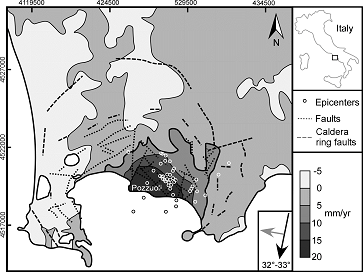
Figure 3: PS-InSAR™showing uplift along the line of sight with data from descending orbit on October 2005–November 2006. Observe the correlation between uplifts, structures, and seismic activity (Modified and synthetized after Vilardo et al., 2010).
Landslide monitoring
Landslides are easily observed because they are moving masses affecting and deforming the relief. As a consequence, the main variables to monitor are the movement and parameters that are modifying the stress or the properties of the material that is under deformation (SafeLand, 2010). Except in the case of earthquakes or exceptional precipitation, the displacement is the main parameter to monitor. In most of the cases, the failure is preceded by an acceleration of movements. Depending on the material, geometry and the volume involved, the failure may be forecasted (Crosta and Agliardi, 2003) and this acceleration can sometime be directly correlated with groundwater levels using a mechanical model (Corominas et al., 2005).
Two types of landslides must be distinguished: shallow and deep-seated landslides. The first are too small and too localized to be easily monitored, but today several attempts are made to create early warnings for shallow landslides (Sassa et al., 2009). The deep-seated failures are usually sufficiently large to display significant movements before catastrophic failure.
Large landslide monitoring
The main instruments used to monitor large landslides are dedicated to movements. Physically, extensometers can be used to measure displacements and crack meters can be used to observe the opening of cracks. When boreholes are available, manual inclinometers or permanent inclinometer columns may be used, providing the deformation profiles and often the failure surface where most of the deformation concentrates. These devices are often used for early warning systems, as for the site of Åknes (Norway) (Blikra, 2008). As water plays an important role in controlling movements of a landslide, boreholes can be used to measure the level of the water table (manually or by measuring the groundwater pressure).
Surface movements can be followed using targets and a total station (laser distance meter), but today, if the required conditions of visibility are appropriate, permanent GNSS can be used for a permanent monitoring of the movements (Gili et al., 2000). The disadvantage of these methods is that they are point measurements only. By using advanced satellite InSAR techniques (PS-InSAR, SBAS, etc), a significant percentage of landslides can be imaged and monitored. In addition, time series of displacement of ground reflectors can be obtained. One of the last evolutions of the InSAR is the SqueeSARTM method that enhances significantly the capability of tracking ground displacement (Ferretti et al., 2011). Unfortunately, satellite InSAR is not suitable for early-warning because satellites take several days to pass over an area a second time. If no appropriate reflective object exists on the monitored surface (for instance due to forest cover), the InSAR method can be applied only if corner reflectors are installed on the ground, providing movements on selected points only (Singhroy et al., 2011). With Ground Based – InSAR (GB-InSAR), it is possible to follow the movements of the surface of a landslide or rockslide, when it is visible in the direction of the line of sight. This is very useful to observe the deformation evolution of the front of landslides (Tarchi et al., 2003).
The Lidar technique provides full 3D point clouds in the case of terrestrial Laser scanner (TLS), which allows characterizing rock slopes and landslides (Safeland, 2010; Jaboyedoff et al., 2012). It permits to monitor and to follow the full evolution of a landslide surface that is moving, to understand mechanisms of failure (Oppikofer et al., 2008) and also to monitor rock falls by comparison of successive acquisitions (Figure 4). The airborne Laser scanner (ALS) is less accurate but permits to estimate differences between digital elevation models.
For most landslides, several different sensors are required to establish an early-warning system (Blikra, 2008; Froese and Moreno, 2011). Since a few years ago, photogrammetry and image correlation have developed, leading to very promising results (Traveletti et al., 2012). Geophysical methods are also improving their capabilities to image the underground. One of the most interesting recent developments is ambient seismic noise analysis. For a rock mass, it indicates a decrease of the natural frequency before failure and for landslides, a decrease of the surface wave velocity (Mainsant et al., 2012).
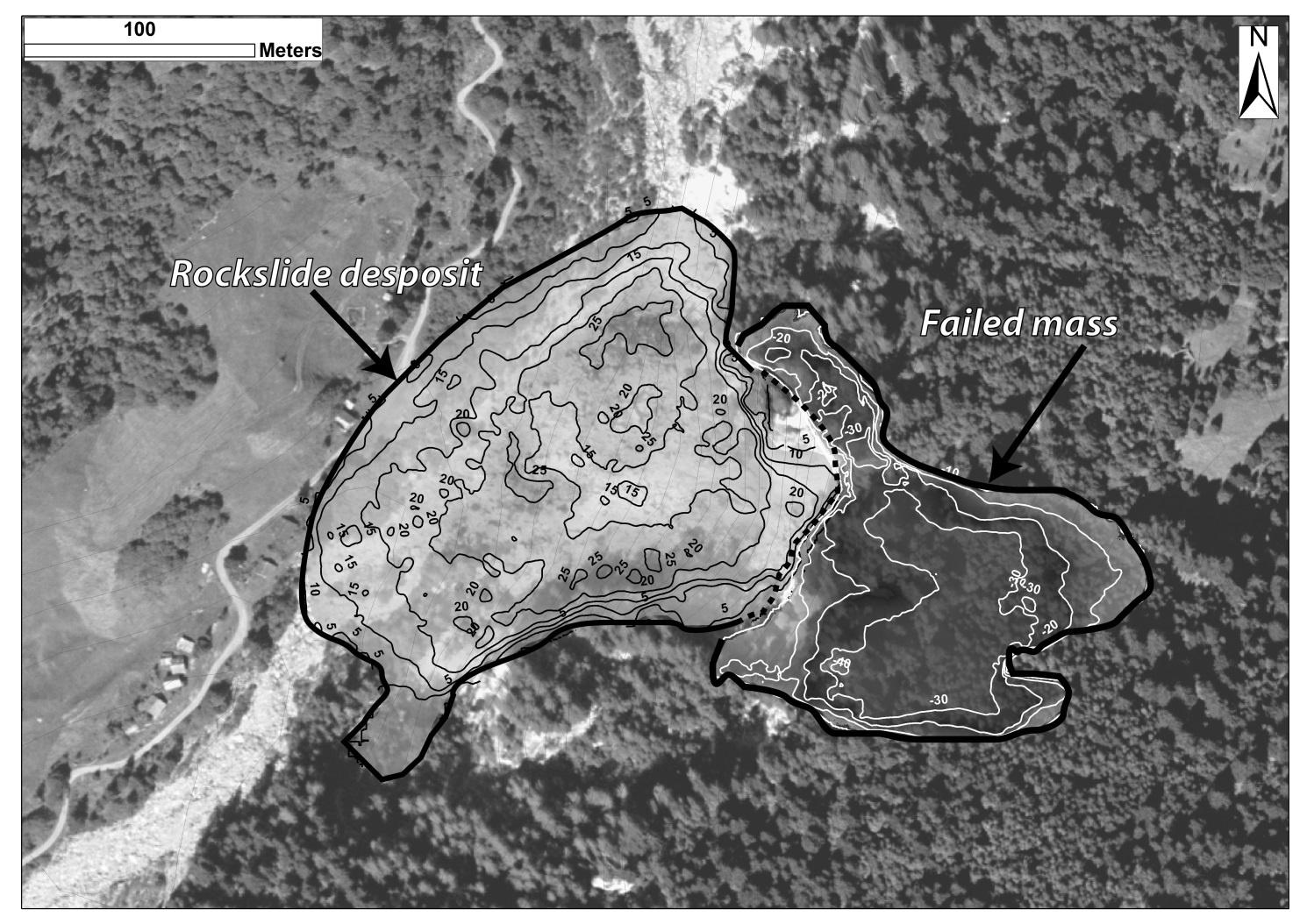
Figure 4: Map of the deposit and failed mass thickness of the of the Val Canaria rockslide (Ticino, Southern Swiss Alps). This map based on the comparison of the airborne and terrestrial Lidar digital elevation model taken before and after the 27.10.2009 rockslide event (modified after Pedrazzini et al., 2011; the aerial picture and airborne Lidar are provided by swisstopo).
Debris flow and shallow landslides monitoring
Shallow landslides and debris-flow landslides are mostly dependent on precipitation. As a consequence, the main monitored variables are precipitation intensity and duration (Baum and Godt, 2010; Jakob et al., 2011). Saturation, soil moisture and antecedent precipitation are variables that are also often monitored. In the case of shallow landslides, the exact location cannot be determined, thus the entire area is considered as hazardous if some thresholds are exceeded. It must be noticed that an early warning system designed for rainfall-induced landslides is operational in Hong-Kong and has been continuously improved since 1977 (Chan et al., 2003; Sassa et al., 2009).
In the case of debris-flows, sensitive catchments can be equipped in order to issue warnings. The seismic sensors and ultrasonic gauges permit one to deduce velocity and peak discharge (Marchi et al., 2002).
Monitoring shallow landslides and debris flows is still a topic of research under development, because the triggering and the localisation of such phenomena are not yet well understood.
Snow avalanche monitoring
Snow avalanches are seasonal events and depend strongly on climate variables such as previous precipitation, snowpack depth and strength and temperatures. As a consequence, snow avalanches monitoring concentrates essentially on hazard level quantification. This is mainly performed using human observations (SLF, 2012) and weather stations equipped by ultrasonic snow depth sensors. Observed variables are strongly dependant on local physiographic conditions. In addition to monitored data, the observers perform snow hardness tests in order to detect the potential mechanical weakness in the snowpack (Pielmeier and Schneebeli, 2002). The conditions for avalanches are so diverse (wet snow, large amount of fresh snow, etc.), that up to now, human intervention in the monitoring remains the main method to monitor and forecast this hazard.
Other monitoring
There are other hazards to monitor. Some require the integration of meteorological data in the monitoring design. For instance, a drought corresponds to a period of abnormally dry weather leading to a deficit of water in the hydrologic cycle and finally leading to problems (but the definition of drought is not unique). Forest fires are consequences of dryness, with origins that are often not natural, but anthropogenic. Hail storms are also hazardous phenomenon that can lead to serious damage; hail monitoring is mainly based on human observation and meteorological radar. Lightning are monitored using a network of electromagnetic sensors. All the sensors detecting one specific lightning provide the distance to it. The location is then deduced by searching the best agreement between all the detected distances to the sensors.
Future of monitoring as a demand of society
The monitoring of natural hazards is often a tedious task, because if the physics well describes the single phenomenon, in natural environments, the occurrence of an event is controlled by several simultaneous phenomena. It implies that, for the analysis and prediction of events, a number of different variables are required, to be able to describe all possible cases.
The power of computer science, communication technologies and the improving quality of sensors, combined with decreasing prices, make the monitoring of environmental data more precise and easy. This leads to a new understanding of natural hazards and also to the implementation of early-warning systems that will permit one to manage territories in a safer way. In addition nowcasting, as proposed by World Meteorological Organization, is now an objective of this organisation to provide forecasts in less than 6 hours. Such developments are mainly possible because of computer power available almost everywhere and a generalized ability to communicate rapidly by anybody with the ‘smartphone’ technology.
References
Austin, G. L., and Bellon, A., 1974. The use of digital weather radar records for short-term precipitation forecasting. Quarterly Journal of the Royal Meteorological Society, 100(426): 658-664
Baum, R. L. and Godt, J. W., 2010. Early warning of rainfall-induced shallow landslides and debris flows in the USA. Landslides, 7, 259-272. DOI 10.1007/s10346.
Blikra L.H., 2008. The Åknes rockslide; monitoring, threshold values and early-warning. In Chen Z, Zhang J, Li Z, Wu F, Ho K. (Eds.) Landslides and Engineered Slopes, From Past to Fu-ture. Proceedings of the 10th International Symposium on Landslides. Taylor and Francis Group. P. 1089–1094.
Brenguier, F., Shapiro, N., Campillo, M., Ferrazzini, V., Duputel, Z.,Coutant, O., and Nercessian, A., 2008. Towards forecasting volcanic eruptions using seismic noise. Nature Geoscience, 1: 126-130
Brown, R., Lemon, L., and Burgess, D., 1978. Tornado detection by pulsed doppler radar. Monthly Weather Review, 106: 29-38
Chan, R.K.S., Pang, P.L.R., Pun, W.K. 2003. Recent developments in the landslips warning system in Hong Kong. In: Ho KKS, Li KS (eds.) Geotechnical engineering—meeting society’s needs: proceedings of the 14th Southeast Asian Geotechnical Conference, Hong Kong. Balkema, Rotterdam, pp. 219–224
Corominas, J., Moya, J., Ledesma, A., Lloret, A. Gili, J.A, 2005. Prediction of ground displacements and velocities from groundwater level changes at the Vallcebre landslide (Eastern Pyrenees, Spain). Landslides, 2, 83-96.
Costa, J. E., R. T. Cheng, F. P. Haeni, N. Melcher, K. R. Spicer, E. Hayes,W. Plant, K. Hayes, C. Teague, and D. Barrick 2006. Use of radars to monitor stream discharge by noncontact methods, Water Resour. Res., 42, W07422, doi:10.1029/2005WR004430.
Crosta G. and Agliardi F. 2003. Failure forecast for large rock slides by surface displacement measurements. Can. Geotech. J., 40, 176-191.
Daley, R., 1993. Atmospheric Data Analysis, Cambridge University Press.
Donaldson, R. J., 1970. Vortex signature recognition by a doppler radar. Journal of Applied Meteorology, 9: 661-670
Durant, A. J., Bonadonna, C., and Horwell, C. J., 2010. Atmospheric and environmental impacts of volcanic particulates. Elements, 6: 235-240
Ferretti A., A. Fumagalli, F. Novali, C. Prati, F. Rocca and A. Rucci. 2011. A New Algorithm for Processing Interferometric Data-Stacks: SqueeSAR, IEEE Transactions on Geoscience and Remote Sensing, 49, 3460 – 3470.
Froese, C.R. and Moreno, F. 2011. Structure and components for the emergency response and warning system on Turtle Mountain. Natural Hazards, doi: 10.1007/s11069-011-9714-y.
Germann, U., Galli, G., Boscacci, M., and Bolliger, M., 2006. Radar precipitation measurement in a mountainous region. Quarterly Journal of the Royal Meteorological Society, 132: 1669-1692
Gili, J.A. , Corominas, J. and Rius J. 2000. Using GlobalPositioning System techniques in landslide monitoring. Eng. Geo., 55, 167–192.
Gleckler, P. J., Wigley, T. M. L., Santer, B. D., Gregory, J. M., AchutaRao, K., and Taylor, K. E., 2006. Volcanoes and climate: Krakatoa’s signature persists in the ocean. Nature, 439: 675
Griffith, C., Woodley, W., Grube, P., Martin, D., Stout, J., and Sikdar, D., 1978. Rain estimation from geosynchronous satellite imagery-visible and infrared studies. Monthly Weather Review, 106(8): 1153-1171
Heki, K., 2011. Ionospheric electron enhancement preceding the 2011 Tohoku‐ Oki earthquake. Geophysical Research Letters, 38: L17312
Hyndman, R. D., and Wang, K., 1995. The rupture zone of Cascadia great earthquakes from current deformation and the thermal regime, Journal of Geophysical Research, 100(B11): 22,133-22,154
Igarashi, G., Saeki, S., Takahata, N., Sumikawa K., , Tasaka, S., Sasaki, Y., Takahashi, M., and Sano, Y., 1995. Ground-water radon anomaly before the Kobe earthquake in Japan. Science, 269: 60-61
Iguchi, T., Meneghini, R., Awaka, J., Kozu, T. and Okamoto, K., 2000. Rain profiling algorithm for TRMM precipitation radar data. Advances in Space Research, 25(5), 973-976.
Jaboyedoff, M., Oppikofer, T., Abellán, A., Derron, M.-H., Loye, A., Metzger, R., Pedrazzini, A. 2012. Use of LIDAR in landslide investigations: a review. Natural Hazards, 61:5–28, DOI 10.1007/s11069-010-9634-2.
Jakob, M., Owen, T. and Simpson, T., 2011. A regional real-time debris-flow warning system for the District of North Vancouver, Canada. Landslides, doi:10.1007/s10346-011-0282-8.
Jensen, J.R., 2007. Remote Sensing of the Environment: An Earth Resource Perspective, 2nd Ed., NJ: Prentice Hall.
Ji, C., Wald, D.J., and Helmberger, D.V., 2002. Source description of the 1999 Hector Mine, California, Earthquake, Part I: Wavelet domain inversion theory and resolution analysis, Bulletin of the Seismological Society of America, 92(4): 1192-1207
Joseph, A. 2011. Tsunamis: Detection, Monitoring, and Early-Warning Technologies. Academic Press.
Kalnay, E., 2003. Atmospheric modeling, data assimilation, and predictability, Cambridge University Press.
Kawanishi, T., Kuroiwa, H., Kojima, M., Oikawa, K., Kozu, T., Kumagai, H., Okamoto, K., Okumura, M., Nakatsuka, H. and Nishikawa, K., 2000. TRMM Precipitation Radar. Advances in Space Research, 25(5): 969-972
Kuo T, Fan K, Kuochen H, Han Y, Chu H, Lee Y., 2006. Anomalous decrease in groundwater radon before the Taiwan M6.8 Chengkung earthquake. J. Environ. Radioact., 88, 101-6.
Landsea C.W, 2007. Counting Atlantic Tropical Cyclones Back to 1900. EOS transactions Amer. Geophys. Union, 88 (18), 197-202.
Mainsant G., Larose E., Brönnimann C., Jongmans D., Michoud C., Jaboyedoff M. 2012. Ambient seismic noise monitoring of a clay landslide: toward failure prediction. JGR-ES, 117, F01030, 12 PP. doi:10.1029/2011JF002159.
Malardel, S. 2005. Fondamentaux de météorologie. À l’école du temps, Toulouse: Cépaduès.
Marchi, L., Arattano, M. and A.M. Deganutti, 2002. Ten years of debris-f low monitoring in the Moscardo Torrent (Italian Alps). Geomorphology, 46, 1 – 17.
Massonet D., Briole, P., and Arnaud, A., 1995. Deflation of Mount Etna monitored by spaceborne radar interferometry. Nature, 375: 567-570
McNutt, S. R., Rymer, H., and Stix, J., 2000. Synthesis of Volcano Monitoring, Chapter 8 of Encyclopedia of Volcanoes, San Diego: Academic Press, pp. 1165-1184
Meinig, C., S.E. Stalin, A.I. Nakamura, F. González, and H.G. Milburn 2005. Technology Developments in Real-Time Tsunami Measuring, Monitoring and Forecasting. In Oceans 2005 MTS/IEEE, 19–23 September 2005, Washington, D.C.
Minnett, P.J., Evans, R.H., Kearns, E.J., Brown, O.B. 2002. Sea-surface temperature measured by the Moderate Resolution Imaging Spectroradiometer (MODIS) Geoscience and Remote Sensing Symposium, 2002. IGARSS ’02. 2002 IEEE, 2, 1177-1179.
NASA, 2012a. Temperature. National Aeronautics and Space Administration, https://science.nasa.gov/earth-science/oceanography/physical-ocean/temperature, visited in May 2012.
NASA, 2012b. https://earthobservatory.nasa.gov/, visited in May 2012.
Nerem, R. S., Chambers, D., Choe, C., and Mitchum G. T. 2010. Estimating Mean Sea Level Change from the TOPEX and Jason Altimeter Missions. Marine Geodesy, 33: 435- 446.
NOAA 2012. https://www.ndbc.noaa.gov/dart.shtml, visited in May 2012.
Olson S.A. and Norris J.M., 2007. U.S. Geological Survey Streamgaging. USGS-Fact Sheet 2005–3131.
Oppikofer, T., Jaboyedoff, M. and Keusen, H.-R. 2008. Collapse of the eastern Eiger flank in the Swiss Alps. Nature Geosciences, 1, 531-535.
Pedrazzini A., Abellan A. Jaboyedoff M. and Oppikofer T. 2011. Monitoring and failure mechanism interpretation of an unstable slope in Southern Switzerland based on terrestrial laser scanner. 14th Pan-American Conference on Soil Mechanics and Geotechnical Engineering.
Pielmeier, C., Schneebeli, M., 2002. Snow stratigraphy measured by snow hardness and compared to surface section images. In Proceedings of the Int. Snow Science Workshop 2002, Penticton, B.C., Canada, pp. 345-352.
Prata, A.J. 2009. Satellite detection of hazardous volcanic clouds and the risk to global air traffic. Natural Hazards, 51, 303 -324
RCPEVE, 2012. The 2011 off the pacific coast of Tohoku Earthquake (M9.0). Research Center for Prediction of Earthquakes and Volcanic Eruptions, https://www.aob.geophys.tohoku.ac.jp/aob-e/info/topics/20110311_news/index_html, visited in May 2012.
SafeLand, 2010. deliverable 4.1 – Review of Techniques for Landslide Detection, Fast Characterization, Rapid Mapping and Long-Term Monitoring. Edited for the SafeLand European project by Michoud C., Abellán A., Derron M.-H. and Jaboyedoff M. Available at https://www.safeland-fp7.eu.
Sassa, K., Picarelli, L. and Yueping, Y. 2009. Monitoring, Prediction and Early Warning. In: Chapter 20 in Sassa, K.. and Canuti, P. (Eds.) Landslides- Distater risk reduction. Springer. 351-375.
Schär C, Vidale PL, Lüthi D, Frei C, Häberli C, Liniger MA, Appenzeller C. 2004. The role of increasing temperature variability in European summer heatwaves. Nature, 427(6972), 332-6.
Shaw, E. 1994. Hydrology in Practice (3rd ed.). Chapman & Hall, London.
Shuttleworth., W. J., 2012. Terrestrial hydrometeorology, Chichester: Wiley-Blackwell.
Singhroy V., Charbonneau F., Froese C., Couture R. 2011. Guidelines for InSAR Monitoring of Landslides in Canada. 14th Pan-American Conference on Soil Mechanics and Geotechnical Engineering.
SLF, 2012. https://www.slf.ch/lawineninfo/zusatzinfos/howto/index_EN, visited in May 2012.
Smith W.H.F., Scharroo R., Titov V.V., Arcas D., Arbic B.K. 2005. Satellite Altimeters Measure Tsunami. Oceanography, 18, 10-12.
Stein, R. S., Barka, A. A., and Dieterich, J.H., 1997. Progressive failure on the North Anatolian fault since 1939 by earthquake stress triggering. Geophysical Journal International, 128: 594-604
Tarchi D., N. Casagli, R. Fanti, D. Leva, G. Luzi, A. Pasuto, M. Pieraccini and S. Silvano. 2003. Landside Monitoring by Using Ground-Based SAR Interferometry: an example of application to the Tessina landslide in Italy. Eng. Geo., 68, 15-30.
Travelletti, J., Delacourt C., Allemand, P., Malet J.-P. Schmittbuhl, J., Toussaint, R., Bastard, M. 2012. Correlation of multi-temporal ground-based optical images for landslide monitoring: Application, potential and limitations. ISPRS Journal of Photogrammetry and Remote Sensing, 70, 39–55.
UNOSAT, 2012. https://www.unitar.org/unosat/node/44/1259, visited in May 2012.
Vicente, G., Scofield, R. and Menzel, W., 1998. The operational goes infrared rainfall estimation technique. Bulletin of the American Meteorological Society, 79(9): 1883-1898
Vilardo, G., Isaia, R., Ventura, G., De Martino, P., Terranova, C. 2010. InSAR Permanent Scatterer analysis reveals fault re-activation during inflation and deflation episodes at Campi Flegrei caldera. Remote Sensing of Env. 114 (2010), 2373–2383.
Wilson, J., Crook, N., Mueller, C., Sun, J. and Dixon, M., 1998. Nowcasting thunderstorms: A status report. Bulletin of the american Meteorological Society, 79(10): 2079-2099.
WMO 2012a https://www.wmo.int/pages/themes/weather/index_en.html, visited in May 2012.
WMO 2012b. https://www.wmo.int/pages/about/Resolution40_en.html, visited in May 2012.